The basic idea in Lagrangian duality is to take the constraints into account by augmenting the objective function with a weighted sum of the constraint functions.
💡
By using the Lagrangian, we can get a hint to solve the original problem which is not convex nor easy to solve.
Standard form problem (not necessary convex)
minimize f0(x)
subject to
fi(x)≤0i=1,…,mhi(x)=0i=1,…,p
where x∈Rn, domain D, optimal value p∗
Lagrangian
L(x,λ,ν)=f0(x)+i=1∑mλifi(x)+i=1∑pνihi(x)
where L:Rn×Rm×Rp→R with dom L=D×Rm×Rp
💡
We call λ,ν as a dual variable or Lagrange multipliers
Since the dual function is the point-wise infimum of a family of affine functions of (λ,μ), it is a concave function. This is because we can view this problem as a point-wise supremum problem by adding a negative term to our objective function. Even though we add a negative term, it is still affine on (λ,μ) (i.e it satisfies the convexity on (λ,μ) for fixed x)
💡
When the Lagrangian is unbounded below in x, the dual function takes on the value −∞
Proof
We already know that convexity preserving operations.
If f(x,y) is convex in x for every y∈A, then
g(x)=y∈Asupf(x,y)
is convex
Since L(x,λ,ν) is concave in (λ,ν) for every x∈D, then
x∈DinfL(x,λ,ν)
is concave.
lower bound property
If λ⪰0, then g(λ,ν)≤p∗
Proof
If xˉ is feasible and λ⪰0, then
f0(xˉ)≥L(xˉ,λ,ν)≥x∈DinfL(x,λ,ν)=g(λ,ν)
minimizing over all feasible xˉ gives p∗≥g(λ,ν)
Example
Least-norm solution of linear equations
minimize xTx
subject to
Ax=b
Dual function
Lagrangian is L(x,ν)=xTx+νT(Ax−b)
to minimize L over x, set gradient equal to zero
∇xL(x,ν)=2x+ATν=0
Therefore,
x=−21ATν
plug in to L to obtain g
g(ν)=L((−1/2)ATν,ν)=−41vTAATν−bTν
a concave function of ν
lower bound property
p∗≥−(1/4)νTAATν−bTν
for all ν
💡
It might seem useless at a first glance, but it is really useful. Let’s say we have a million equality constraints above. In this case, it is impossible to use analytical solution directly. Instead, we have to use iterative approach. Then we have to decide when should we stop. In this situation, we can use the lower bound.
Therefore, we can interpret Wij as a measure of hostility since if Wij is large, we have to allocate the opposite sign to xi and xj respectively.
In this case, we already know the conjugate of f0
The Lagrange dual problem
For each pair (λ,ν) with λ⪰0, the Lagrange dual function gives us a lower bound on the optimal value p∗ of the optimization problem. Thus we have a lower bound that depends on some parameters λ,ν.
The natural question is: What is the best lower bound that can be obtained from the Lagrange dual function?
This leads to the optimization problem
maximize g(λ,ν)
subject to
λ⪰0
This problem is called the Lagrange dual problem. The term dual feasible, to describe a pair (λ,ν) with λ⪰0 and g(λ,ν)>−∞.
💡
Note that the Lagrange dual problem is a convex optimization problem that doesn’t depend on the convexity of the original problem since the objective function to be maximized is concave and the constraint is convex
Example
standard form LP and its dual
standard form
minimize cTx
subject to
Ax=bx⪰0
dual problem
maximize −bTν
subject to
ATν+c⪰0
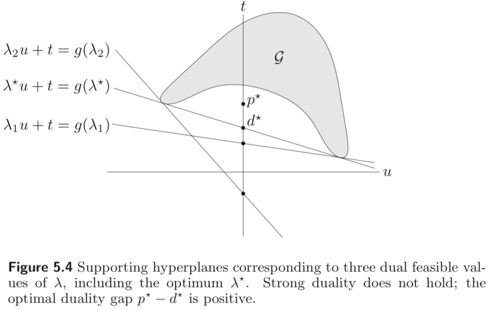
Weak and strong duality
weak duality : d∗≤p∗ (where d∗ is the optimal value of the dual problem)
it always hold for convex and non-convex problems.
it can be used to find non-trivial lower bounds for difficult problem
strong duality : d∗=p∗
it does not hold in general
(usually) holds for convex problems
conditions that guarantee strong duality in convex problems are called constraint qualifications
Slater’s constraint qualification
One simple constraint qualification is Slater's condition
Let our problem is as follows
minimize f0(x)
subject to
fi(x)≤0i=1,…,mAx=b
where f0,…,fm is a convex function.
If there exists an x∈relint D such that
fi(x)<0i=1,…,mAx=b
Such a point is sometimes called strictly feasible
Slater’s theorem states that strong duality holds if Slater’s condition holds and the problem is convex.
💡
Slater’s condition must require the convexity of the problem
Therefore, the two inequalities holds with equality.
So, x∗ minimizes L(x,λ∗,ν∗) and
λi∗fi(x∗)=0i=1,…,m
More specifically,
λi∗>0⇒fi(x∗)=0fi(x∗)<0⇒λi∗=0
It is known as complementary slackness
Karush-Kuhn-Tucker (KKT) conditions
We now assume that the functions fi,hi are differentiable and therefore have open domains.
Let x∗ and (λ∗,ν∗) be any primal and dual optimal points with zero duality gap. Since x∗ minimizes L(x,λ∗,ν∗) over x, it follows that its gradient must vanish at x∗
∇f0(x∗)+i=1∑mλi∗∇fi(x∗)+i=1∑pνi∗∇hi(x∗)=0
Thus the KKT conditions is as follows
primal constraints
fi(x∗)≤0i=1,…,mhi(x∗)=0i=1,…,m
dual constraints
λ∗⪰0
💡
Note that there is no constraint on ν.
complementary slackness
λifi(x∗)=0i=1,…,m
stationary
∇f0(x∗)+i=1∑mλi∗∇fi(x∗)+i=1∑pνi∗∇hi(x∗)=0
if strong duality holds and x∗,λ∗,ν∗ are optimal, then they must satisfy the KKT conditions.
💡
In other words, if strong duality holds, KKT conditions hold for any pair of primal optimal and dual optimal
💡
Note that it is possible that even though x,λ,ν satisfy the KKT conditions, we can't guarantee that it is an optimal point for primal and dual problems respectively.
KKT conditions for convex problems
When the primal problem is convex, the KKT conditions are also sufficient for the points to be primal and dual optimal. In other words, if fi are convex and hi are affine, and x~,λ~,ν~ are any points that satisfy the KKT conditions, then x~ and (λ~,ν~) are primal and dual optimal, with zero duality gap.
Since λ~i≥0, L(x,λ~,ν~) is convex in x. Moreover, from the complementary slackness condition, x~ minimizes L(x,λ~,ν~) over x.
This shows that x~ and (λ~,ν~) have zero duality gap, and therefore are primal and dual optimal.
💡
For any convex optimization problem with differentiable objective functions, any points that satisfy the KKT conditions are primal and dual optimal, and have zero duality gap
💡
For convex problems, primal and dual optimality satisfy if and only if KKT condition holds
💡
But we can not guarantee that we can always find (x~,λ~,ν~) that satisfy the KKT conditions. We can just say that if we find that point, it is primal and dual optimal respectively.
KKT conditions for convex problems with Slater’s condition
If a convex optimization problem with differentiable objective and constraint functions satisfies Slater’s condition, then the KKT conditions provide necessary and sufficient conditions for optimality. Since Slater’s condition implies that the optimal duality gap is zero and the dual optimum is attained, so if x is optimal we can always find (λ,ν) that satisfy the KKT conditions.
💡
Of course, if we find (x,λ,ν) satisfy the KKT conditions, we can guarantee that x is an optimal point in a primal problem and (λ,ν) is an optimal point in a dual problem.
Example : Water-filling
Assume αi>0 (αi is a given value)
minimize −i=1∑nlog(xi+αi)
subject to
x⪰01Tx=1
💡
Note that it is a convex optimization problem that satisfies the Slater’s condition
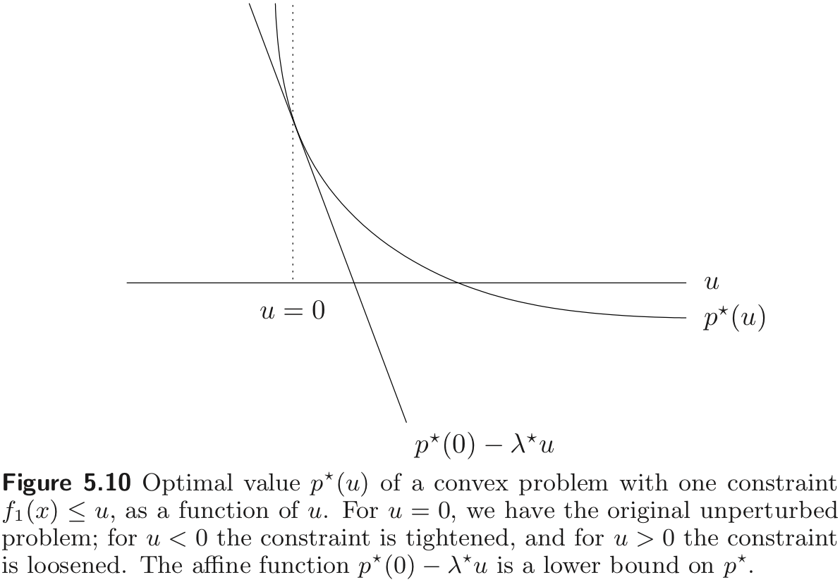
When strong duality holds, the optimal dual variables give very useful information about the sensitivity of the optimal value with respect to perturbations of the constraints.
💡
For some problems, it is easier to solve a dual problem rather than a primal problem. In this case, we can use the optimal dual variable to get information about the primal problem.
Unperturbed optimization problem and its dual
Primal problem
minimize f0(x)
subject to
fi(x)≤0i=1,…,mhi(x)=0i=1,…,p
Dual problem
maximize g(λ,ν)
subject to
λ⪰0
Perturbed problem and its dual
Primal problem
minimize f0(x)
subject to
fi(x)≤uii=1,…,mhi(x)=vii=1,…,p
Dual problem
maximize g(λ,ν)−uTλ−vTν
such that
λ⪰0
💡
It increases the feasible set
where x is a primal variable, u,v are parameters
We define p∗(u,v) as the optimal value of the perturbed problem
p∗(u,v)=inf{f0(x)∣∃x∈D,fi(x)≤ui,hi(x)=vi}
When the original problem is convex, the function p∗ is a convex function of u and v
💡
Whether p∗ is convex or not is benign on the convexity of the original function because x is affected by u and v
Global sensitivity result
Assume that strong duality holds and that the dual optimum is attained. (This is the case if the original problem is convex, and Slater’s condition is satisfied)
Let (λ∗,ν∗) be optimal for the dual of the unperturbed problem. Then for all u and v we have
p∗(u,v)≥g(λ∗,ν∗)−uTλ∗−vTν∗=p∗(0,0)−uTλ∗−vTν∗
💡
The first inequality came from the fact that the dual function value of the perturbed problem is a lower bound of its primal.
We conclude that for any x feasible for the perturbed problem, we have
f0(x)≥p∗(0,0)−uTλ∗−vTν∗
Sensitivity interpretation
If λi∗ is large and we tighten ith constraint (i.e. choose ui<0), then the optimal value p∗(u,v) is guaranteed to increase greatly
If νi∗ is large and positive and we take vi<0, or if νi∗ is large and negative and we take vi>0, then the optimal value p∗(u,v) is guaranteed to increase greatly
If λi∗ is small, and we loosen the ith constraint (ui>0), then the optimal value p∗(u,v) will not decrease too much
If νi∗ is small and positive, and vi>0, or if νi∗ is small and negative and vi<0, then the optimal value p∗(u,v) will not decrease too much.
Local sensitivity
Suppose now that p∗(u,v) is differentiable at u=0,v=0. Then, provided strong duality holds, the optimal dual variables λ∗,ν∗ are related to the gradient of p∗ at u=0,v=0
λi∗=−∂ui∂p∗(0,0)νi∗=−∂vi∂p∗(0,0)
Thus, when p∗(u,v) is differentiable at u=0,v=0, and strong duality holds, the optimal Lagrange multipliers are exactly the local sensitivities of the optimal value with respect to constraint perturbations.
Proof
Since strong duality holds and the dual optimal (λ∗,ν∗) is attained,
The local sensitivity result gives us a quantitative measure of how active a constraint is at the optimum x∗. If fi(x∗)<0, then the constraint is inactive, and it follows that the constraint can be tightened or loosened a small amount without affecting the optimal value since by complementary slackness, the associated optimal Lagrange multiplier must be zero.
But now suppose that fi(x∗)=0. The ith optimal Lagrange multiplier tells us how active the constraint is.
If λi∗ is small : the constraint can be loosened or tightened a bit without much effect on the optimal value
if λi∗ is large : if the constraint is loosened or tightened a bit, the effect on the optimal value will be great
Duality and problem reformulations
Equivalent formulations of a problem can lead to very different duals. Reformulating the primal problem can be useful when the dual is difficult to derive, or uninteresting.
Common reformulations
introduce new variables and equality constraints
make explicit constraints implicit or vice-versa
transform objective or constraint functions
→ replace f0(x) by ϕ(f0(x)) with ϕ convex, increasing
Introducing new variables and equality constraints
Consider an unconstrained problem of the form
minimize f0(Ax+b)
The dual function is constant
g(λ,ν)=xinfL(x,λ,ν)=xinff0(Ax+b)=p∗
We have strong duality, but dual is quite useless.
Since the Lagrangian is affine in the dual variables (λ,ν), and the dual function is a point-wise infimum of the Lagrangian, the dual function is concave.
As in a problem with scalar inequalities, the dual function gives lower bounds on p∗. Similar to λi≥0 the scalar case, it requires the non-negativity requirement on the dual variables for the generalized inequality case.
λi⪰Ki∗0i=1,…,m
where Ki∗ denotes the dual cone of Ki.
Weak duality follows immediately from the definition of dual cone because if λi⪰Ki∗0 and fi(x~)⪯Ki0, then λiTfi(x~)≤0. Therefore for any primal feasible point x~ and any λi⪰Ki∗0 for all i, then
Strong duality holds when the primal problem is convex and satisfies an appropriate constraint qualification as the scalar case such as Slater’s condition.
Example : Semidefinite program
We consider a semi-definite program in inequality form
minimize cTx
subject to
x1F1+⋯+xnFn⪯G
where Fi,G∈Sk. (Here f1 is affine, and K1 is S+k, the positive semi-definite cone.)
Since S+k is self-dual, the Lagrange multiplier Z is in Sk. Then the Lagrangian is
Strong duality obtains if there is a strictly feasible point because it satisfies Slater’s condition. In other words, there exists an x with
x1F1+⋯+xnFn−G≺0
💡
Note that an inner product of two symmetric matrices can be defined as a trace of its multiplication. Check the dual generalized inequality in convex set section.