12. Geometry of Linear Programming

Introduction

Linear programs can be studied both algebraically and geometrically. The two approaches are equivalent, but one or the other may be more convenient for answering a particular question about a linear program.

The algebraic point of view is based on writing the linear program in a particular way, called standard form. Then the coefficient matrix of the constraints of the linear program can be analyzed using the tools of linear algebra.

The geometric point of view is based on the geometry of the feasible region and uses ideas such as convexity to analyze the linear program. It is less dependent on the particular way in which the constraints are written.

Example

Consider the problem

$$\min -x_1 -2x_2$$

$\text{subject to}$

$$-2x_1 + x_2 \le 2 \\ -x_1 + x_3 \le 3 \\ x_1 \le 3 \\ x_1, x_2 \ge 0$$

The feasible region is graphed like this

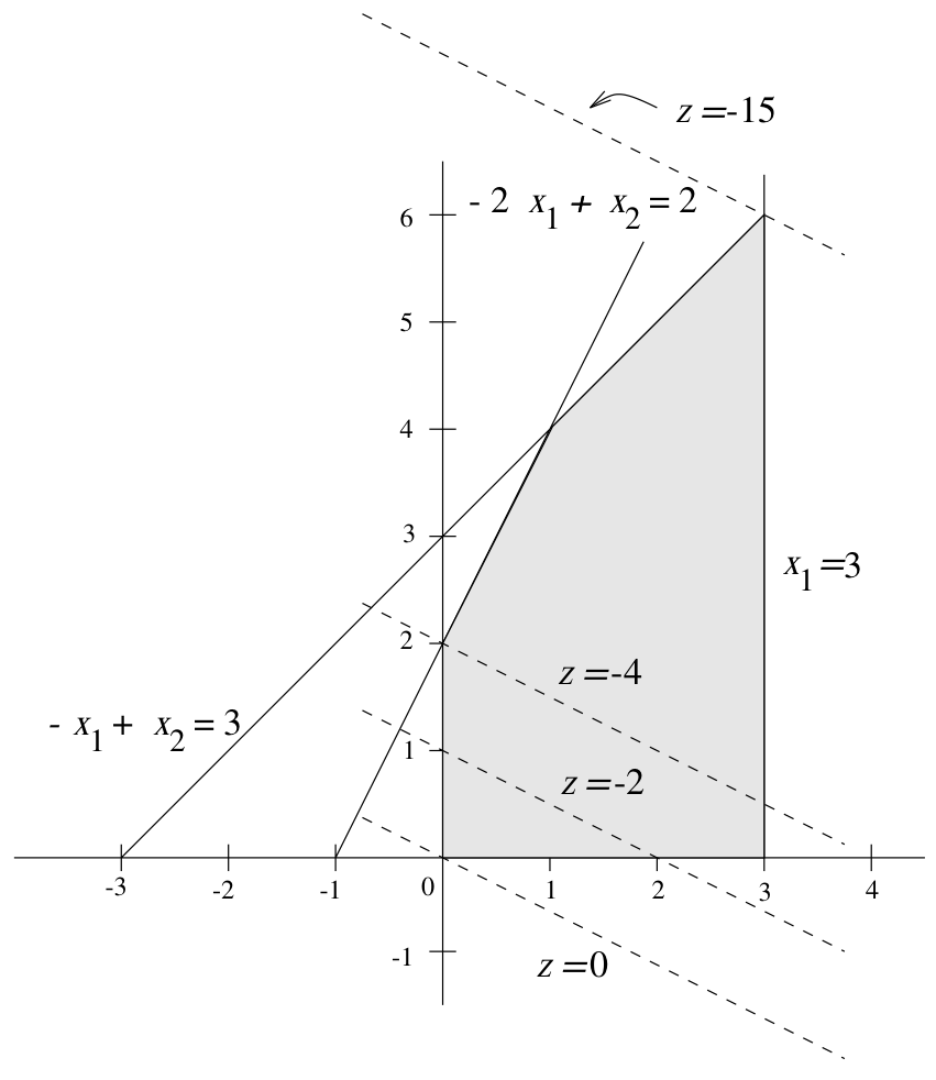
As you can see in the above graph, it has a solution at the corner. But it is no coincidence that the solution occurred at a corner or extreme point.

Standard Form

There are many different ways to represent a linear program. It is sometimes more convenient to use one instead of another. It is called standard form, will be used to describe the simplex method.

In a standard form, it can be represented

$$\min c^Tx$$

$\text{subject to}$

$$Ax= b\\ x\ge 0$$

Note that every linear programming can be transformed into standard form.

From now on, with out any comment, we will assume that $A$ has full rank.

Note that the full-rank assumption is not unreasonable. If $A$ is not a full rank, then either the constraints are inconsistent or there are redundant constraints.

1. If the constraints are inconsistent, then the problem has no solution and the feasible solution is empty.

2. If there are redundant constraints, then theoretically they could be removed from the problem without changing either the solution or the feasible region.

Example

What if we have inequality constraints? In that case, we can easily transform into the standard form by using the slack variable.

For instance,

$$\min -x_1 -x_2$$

$\text{subject to}$

$$-2x_1 + x_2 \ge 2 \\ -x_1 + x_2 \le 3 \\ x_1 \le 3 \\ x_1, x_2 \ge 0$$

This optimization problem can be converted into

$$\min -x_1 -2x_2$$

$\text{subject to}$

$$-2x_1 + x_2 + s_1 = 2 \\ -x_1 + x_2 + s_2 = 3 \\ x_1 + s_3 = 3 \\ x_1, x_2, s_1, s_2, s_3 \ge 0$$

Extreme Points

A point of a vertex set is an extreme point (or vertex) if it can not be expressed using a convex combination of other points. That is

$$v = \alpha x + (1 - \alpha)$$

where $x, y\in S, 0<\alpha <1$

Then,

$$x = y = v$$

In other words, an extreme point is not on the line segment of two different points.

💡

For multiple dimensions, we don’t know which points are extreme points. So we can’t know extreme points in advance.

Representation Theorem

Any non-extreme point $x$ can be expressed using a convex combination of extreme points.

Let $\{v_1, v_2, \dots, v_k\}$ be the set of extreme points of $S$.

Since $x$ is not a extreme point, we can express $x$ as

$$x = \sum_{i = 1}^k \alpha_iv_i$$

where $\alpha_i \ge 0, \sum_{i = 1}^k \alpha_i = 1$

If we transform our original optimization problem into the standard form, our objective function is always like this

$$c^Tx$$

That means,

$$\begin{align} c^Tx &= \sum_{i = 1}^kc^T(\alpha_iv_i) \\ &=\sum_{i = 1}^k \alpha_ic^Tv_i\end{align}$$

Therefore, every non-extreme point can be expressed by linear combination of the extreme points.

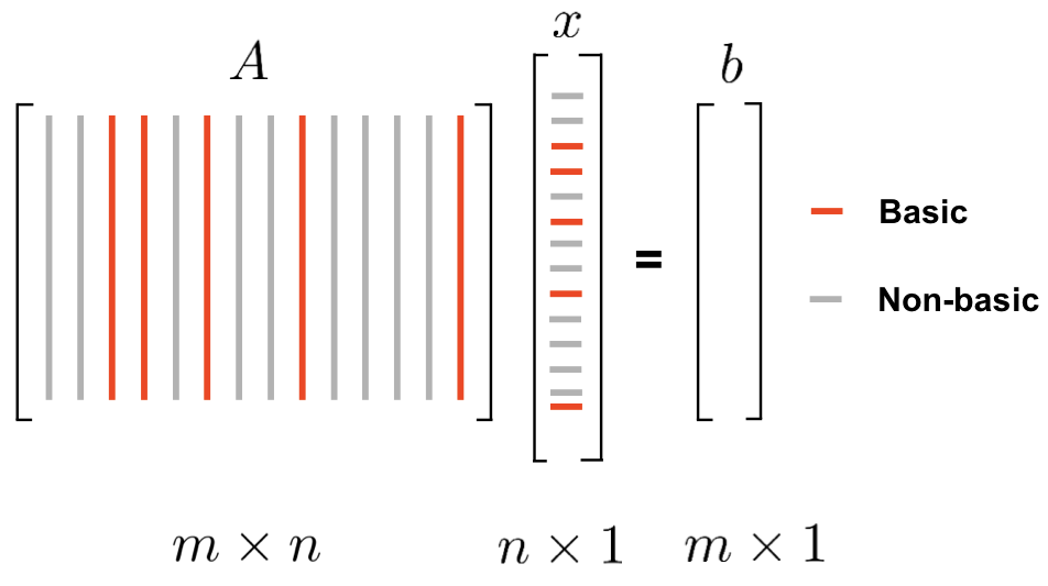
Basic Solutions

A basic solution is defined algebraically using the standard form of the constraints. A point $x$ is a basic solution if

1. $x$ satisfies the equality constraints of the linear program

2. the columns of the constraint matrix corresponding to the nonzero component of $x$ are linearly independent

The set of basic variables is called the basis

If $x \ge 0$, it is called a basic feasible solution (BFS). If is an optimal basic feasible solution if it is also optimal for the linear program.

💡

Note that if a linear program has an optimal solution, then it has an optimal basic feasible solution.

Example

$$\min c^Tx$$

$\text{subject to}$

$$\begin{bmatrix}2 & 1 & 4 \\ 1 & 0 & 5\end{bmatrix}\begin{bmatrix}x_1 \\x_2\\x_3\end{bmatrix} = \begin{bmatrix}1 \\ 2\end{bmatrix}$$

Take $x_3= 0$

$$\begin{bmatrix} 2 & 1 \\ 1 & 0\end{bmatrix}\begin{bmatrix}x_1 \\ x_2 \end{bmatrix} = \begin{bmatrix}1 \\ 2 \end{bmatrix}$$

Extreme Point = BFS

A point $x$ is an extreme point of the set $\{x : Ax = b, x\ge 0\}$ if and only if it is a basic feasible solution.

Proof

Firstly, we show that if $x$ is a feasible solution, then it is a extreme point. W.L.O.G we may assume that the last $n - m$ variables of $x$ are non-basic (if not, we can do so by switching the order of the column of $A$). That is

$$x = \begin{bmatrix}x_B\\x_N\end{bmatrix} = \begin{bmatrix}x_B\\0\end{bmatrix}$$

Let $B$ be the invertible basis matrix corresponding to $x_B$. If $x$ is not an extreme point, then there exist two distinct feasible point $y$ and $z$ such that

$$x = \alpha y + (1 - \alpha)z$$

where $y, z\in S, 0 < \alpha < 1$

Let

$$y = \begin{bmatrix}y_B\\y_N\end{bmatrix}, z = \begin{bmatrix}z_B\\z_N\end{bmatrix}$$

Since $y, z$ are feasible,

$$y_N = z_N = 0$$

Moreover, since $B$ is invertible

$$\begin{align}Bx_B = By_B = Bz_B = b\\ \Rightarrow x_B = y_B = z_B\end{align}$$

However, it contradicts to the assumption. Therefore, $x$ is an extreme point.

Secondly, we prove that if $x$ is an extreme point, then $x$ is a basic feasible point. Let $x$ is a extreme point. That means $Ax = b$ and $x\ge 0$. W.L.O.G $x$ can be written as

$$x = \begin{bmatrix} x_B \\ x_N\end{bmatrix}$$

where $x_B > 0$ and $x_N = 0$. In addition, we can write

$$A = (B, N)$$

where $B$ and $N$ are the coefficient correspoinding to $x_B$ and $x_N$ respectively.

💡

Note that $B$ may not be a square matrix. Therefore, we also can’t guarantee that it is invertible.

If the columns of $B$ are linearly independent, then $x$ is clearly basic solution so that there is nothing to prove.

On the other hand, suppose the columns of $B$ are linearly dependent. Then, there exist $p$ such that

$$B_1p_1 + B_2p_2 + \dots + B_kp_k = 0$$

where $p$ is not zero vector.

In addition, since $x_B$ is positive, we can always find $\epsilon > 0$ such that

$$x_B - \epsilon p > 0 \quad \text{and}\quad x_B + \epsilon p > 0$$

Take

$$y = \begin{bmatrix}x_B - \epsilon p \\ x_N \end{bmatrix}\\ z =\begin{bmatrix} x_B + \epsilon p\\x_N\end{bmatrix}$$

Then, $y$ and $z$ are also feasible point. Moreover

$$x = y + z$$

But it contradicts to the fact that $x$ is a extreme point.

Therefore, $x$ is a basic feasible solution.

Degenerate Solutions

It is possible that one or more of the basic variables in a basic feasible solution will be zero. If this occurs, then the point is called degenerate vertex, and the linear program is said to be degenerate.

Consider the example, with one additional constraint $x_2 \le 6$

$$\min -x_1 -2x_2$$

subject to

$$\begin{align}-2x_1+x_2 + s_1 = 2\\ -x_1 + x_2 + s_2 = 3\\x_1 + s_3 = 3\\x_2 + s_4 = 6\\ x_1, x_2, s_1, s_2, s_3, s_4 \ge 0\end{align}$$

If we take non-basic variable as $s_3$ and $s_4$, we can derive $s_2 = 0$

Additional definitions

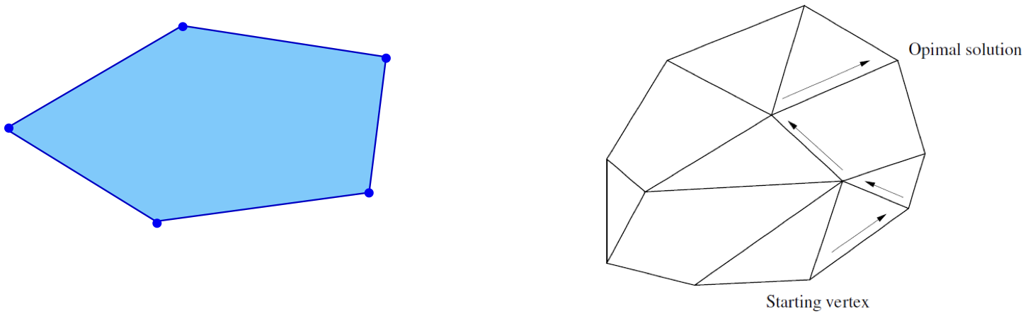
Adjacent Extreme Points

Two extreme points are said to be adjacent if they are connected by an edge of the feasible region. This means there is a direct line or edge that connects the two points within the feasible region.

Adjacent Bases

In a linear programming problem, if you have $m$ equality constraints, two bases are considered adjacent if they share $m - 1$ common variables. Essentially, two bases are adjacent if they agree on most variables and differ in just one.

Adjacent Basic Feasible Solutions

In the context of linear programming, basic feasible solutions (BFS) are solutions that satisfy all constraints of the problem and are located at the vertices of the feasible region. Now, two basic feasible solutions are said to be adjacent if they share all but one of their basic variables.

In other words, if you can move from one BFS to another by just changing one variable (while still remaining within the feasible region), then these two solutions are called adjacent basic feasible solutions. This concept is crucial in the simplex method, as the method involves moving from one BFS to another, improving the objective function at each step, until the optimal solution is reached.

💡

추가적으로 constraint의 수보다 variable의 수가 더 많다고 가정한 상황이므로 full rank라는 것은 surjective를 의미한다.

BFS and Optimality

If a linear program in standard form has a finite optimal solution, then it has an optimal basic feasible solution

💡

It can be prove by using representation theorem.