Computer Science/Optimization
10. Feasible-Point Methods
- -
728x90
반응형
Introduction
In this article, we examine methods that solve constrained optimization problems by attempting to remain feasible at every iteration. If all the constraints are linear, maintaining feasibility is straightforward. However, when non-linear constraints are present, then more elaborate procedures are required. Although it strives to maintain feasibility at every iteration, they do not always achieve this.
Active-set Methods
- Bad news : It can’t be reformulated into unconstrained optimization.
- Good news : We have methods for equality constraints.
How can we resolve this issue? A brute force approach would be to solve the equality-constrained problem for all possible selections of active constraints, and then choose the best solution. However, this approach can’t be applicable even though the number of constraints are quite small.
Active-set methods attempt to overcome this difficulty by moving sequentially from one choice of active constraints to another choice that is guaranteed to produce at least as good a solution.
The most commonly used active-set methods are feasible-point methods. An initial feasible point, if none is provided, can be obtained by using linear-programming. At each iteration of the active-set method, we select a working set of constraints that are assumed to be active at the optimum.
💡
즉, minimizing subject to the constraints를 equality constraint with respect to the working set으로 돌려서 풀겠다는 의미이다.
💡
Note that these are
linear inequality constraints.💡
In general, the working set at the current point is a subset of the constraints that are active at , so that is a feasible point for the working set. There may also be constraints that are active at but that are not included in the working set. Hence the working set is not necessarily equal to the active set.
Algorithm

- Initialize with some working set of active constraints
- Iterate
- Optimality check
- If no constraints are active and the current point is an unconstrained stationary point, then stop
- If there are active constraints and the current point is optimal with respect to the active constraints, compute the Lagrange multipliers
- If the multipliers are non-negative, stop. Otherwise, drop a constraint with negative multiplier from .💡즉, multiplier가 전부 다 양수라는 의미는 gradient 반대 방향이 interior로 절대로 들어오지 않는다는 의미이다. (constraint를 로 잡은 상태이므로 이렇게 해석할 수 있다.). 이 의미는 active constraint에 대해서 optimal이고 interior point로 들어가는 순간 함숫값이 커진다는 의미이므로 local optimum이라고 단정할 수 있는 것이다.
- Search direction
- Determine a descent direction that is feasible with respect to
- Step length
- Determine a satisfying and where is the maximum possible step length along
- Update
- . If new constraint boundary encountered, add to .
- Optimality check
💡
요약하면 working set만을 고려하는 unconstraint optimization problem을 푸는 것처럼 풀고, 나머지 non-working set까지 고려해서 condition이 violated되었는지를 판단하는 것이다.
Example
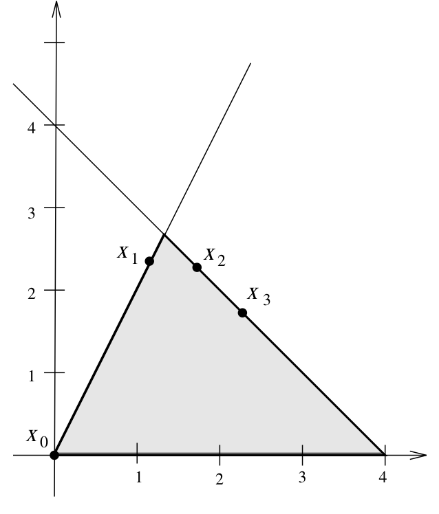
when starting at and

- Active constraints : 1, 3
- Find such that
- Since , the current point is not a optimal point.
- Drop constraint:
- Find the null space
Therefore,
💡Null space 방향을 search direction으로 설정
- Take
- Solve
Since, doesn’t violate the other constraints, it is in the feasible reasion.
- Check the optimality condition again
→ It is also not a optimal point. So we also drop this constraint also
- We are now left with
noactive constraints, which means that the problem is locally unconstrained. Therefore, reduced gradient is simply the unconstrained Newton direction
- Calculate the largest feasible step by considering the given constraints
- Iterate above procedures
Sequential Quadratic Programming (SQP)
Sequential quadratic programming is a popular and successful technique for solving non-linearly constrained problems such as
💡
Active-set method의 경우, linear constraint였음을 잘 기억해야 한다.
The main idea is to obtain a search direction by solving a quadratic program, that is a problem with a quadratic objective function and linear constraints.
💡
This approach is a generalization of Newton’s method for unconstrained minimization
Idea
The Lagrangian for this problem is
and the first-order optimality condition is
Then the formula for Newton’s method is
where and are obtained as the solution to the linear system
💡
This derivation is quite intuitive. If we think the Lagrangian for this problem as a unconstrained optimization problem.
Consider the following the constrained minimization problem where is our Newton iteration at step
💡
Note that the objective function is
quadratic in This minimization problem has Lagrangian
Note that the first optimality condition for above Lagrangian is
which are equivalent to the original first-optimality condition. Then solving gives a linear system, which is the same as the ’th Newton step of the original problem.
The quadratic function is a Taylor series approximation to the Lagrangian at , and the constraints are a linear approximation to
💡
In the constrained case, the formulas for Newton’s method correspond to the constrained minimization of a quadratic approximation to the Lagrangian.
Issue
SQP is an important method, and there are many issues to be considered to obtain an efficient and reliable implementation
- Efficient solution of the lienar system at each Newton iteration
→ block matrix structure can be exploited
- Quasi-Newton approximations to the as in the unconstrained case
- Trust region, line search to improve robustness
- Treatment of constraints (equality and inequality) during the iterative process
- Selection of good starting guess for
반응형
Contents
소중한 공감 감사합니다