Computer Science/Optimization
1. Basics
- -
728x90
반응형
A Generic Optimization Model
In compact form
where ( : the set of all feasible solutions permitted by the constraints)
Assumptions
- Continuous variables, smooth functions (twice continuously differentiable unless stated otherwise)
- Linear programming (LP) and Non-linear programming (NLP)
- What do we mean by solving the problem?
- LP : compute the optimum
- NLP : hard in general; we focus on a
local optimum
Boundary and Interior
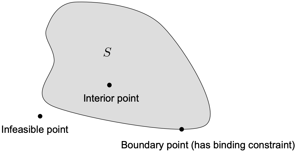
- Boundary of : formed by all feasible points with
at leastone binding constraint; binding = an inequality is satisfied as equality
- Interior of : the rest of , or all feasible points without any binding constraint
Global and Local Optima
- is a global minimum if
- is a local minimum if such that
In general, it is difficult to find the global minimum.
Therefore, we will focus on finding a local minimum in nonlinear optimization problems.
How to Solve it?
- Take a sequence of steps to improve the objective function
- Convergence : A point that is locally optimal
General Algorithm
- Specify some initial guess of the solution
- For k = 0, 1, …
- If is locally optimal, stop
- Determine a search direction
- Determine a step length , such that is a better solution than
💡
Technically, we have to consider about the shape at the point.
Descent Direction
- It is desirable to have descent direction as our search direction
- Formal definition
A direction of function at point is a descent direction, if there exists such that
Note
Any direction less than from is a descent direction
Hessian
Second-order derivative of a function in several variables is called the Hessian
The Hessian is a square and symmetric matrix
It is useful for optimality check, and function approximation.
Taylor Series
- One dimension
- Multiple dimensions
What about approximating at point with and find the best possible for the approximation?
What about adding one more term in the approximation?
Sensitivity (Conditioning)
- There may be errors in the input data
- Also, data calculations are not completely accurate by computers
- Intuitively, we have an ill-conditioned problem if the solution is very sensitive to the change of data values
💡
A singular matrix has condition number .
반응형
Contents
소중한 공감 감사합니다