7. Support Vector Machine

Functional Margin and Geometric Margin

What is the difference

The key difference between the functional margin and geometric margin is that the functional margin is defined for every data point, whereas the geometric margin is defined only for the data point closest to the decision boundary. The geometric margin is often used as a measure of the generalization performance of a linear classifier, as it captures how well the classifier can separate new data points that are similar to the training data.

Functional Margin

Given a training example $(x^{(i)}, y^{(i)})$, we define the functional margin of $(w, b)$ with respect to the training example

$$\hat r^{(i)} = y^{(i)}(w^Tx + b)$$

Note that if $y^{(i)} = 1$, then for the functional margin to be large (i.e. for our prediction to be confident and correct), we need $w^Tx + b$ to be a large positive number. Conversely, if $y^{(i)} = -1$, then for the functional margin to be large, we need $w^Tx + b$ to be a large negative number.

💡

$y^{(i)}(w^Tx + b) > 0$ means that our prediction on this example is correct. (i.e. a large functional margin represents a confidentand a correct prediction

Given a training set $S = \{(x^{(i)}, y^{(i)})| i = 1, \dots, m\}$, we can define the functional margin of $(w, b)$ with respect to S to be the smallest of the functional margins of the individual training examples. Denoted by $\hat r$, this can be written as

$$\hat r = \min_{i = 1, \dots, m}\hat r^{(i)}$$

However, there’s one property of the functional margin that makes it not a very good measure of confidence. This is because if we replace $w$ with $2w$ and $b$ with $2b$, then since $g(w^Tx + b) = g(2w^t+2b)$, this would not change the result of classifier (Since, classifier and $g$ depends only on the sign, but not on the magnitude.

💡

where $g(z) = 1$ if $z\ge 0$, and $g(z) = -1$ otherwise

This means that we can scale $w$ and $b$ without changing the result of classifier. Intuitively, it might therefore makes sense to impose some sort of normalization condition such as $\|w\|_2 = 1$ (i.e. we can replace $w$ and $b$ with $w/\|w\|_2$ and $b/\|w\|_2$ respectively. So the concept of geometric margin arises.

Geometric margin

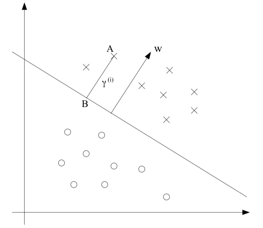
We want to show that geometric margin is not only the normalizing functional margin but also the actual geometric distance between the datapoint and the decision boundary. Since we already know that $A$ represents $x^{(i)}$, we therefore find that the point $B$ is given $x^{(i)} - r^{(i)}\cdot w/\|w\|$. In addition, we already know that the point $B$ lies in the decision boundary. Therefore

$$w^T(x^{(i)}=r^{(i)}\frac{w}{\|w\|}) + b = 0$$

Solving for $r^{(i)}$ yields

$$r^{(i)} = (\frac{w}{\|w\|})^Tx^{(i)} + \frac{b}{\|w\|}$$

💡

Therefore, the geometric margin must be interpreted as a normalized functional margin and the geometric distance between datapoints and the decision boundary.

Therefore, the geometric margin is invariant to rescaling of the parameters.

In addition, given a training set $S = \{(x^{(i)}, y^{(i)})| i = 1, \dots, m\}$, we also define the geometric margin of $(w, b)$ with respect to $S$ to be the smallest of the geometric margins on the individual training examples:

$$r = \min_{i = 1, \dots, m}r^{(i)}$$

The optimal margin classifier

Given a training set, we want to find the optimal decision boundary that maximizes the geometric margin. We will assume that we are given a training set that is linearly separable.

💡

If the training set that is not linearly separable, it can be solvable by using regularization. This concept will discuss later.

So, we want to solve the following optimization problem

$$\max_{r, w, b}r \\ \text{subject to }y^{(i)}(w^Tx^{(i)} + b) \ge r, i = 1,\dots, m \\ \text{and } \|w\|=1$$

But this optimization problem has “$\|w\| = 1$” constraint which is not a convex. So, we have to reformulate the above optimization problem as follows

$$\max_{\hat r, w, b}\frac{\hat r}{\|w\|} \\ \text{subject to }y^{(i)}(w^Tx^{(i)} + b) \ge \hat r, i = 1,\dots, m \\$$

However, the objective function($\frac{\hat r}{\|w\|}$) still non-covex function, so we need to step further. Recall our earlier discussion that we can add an arbitrary scaling constraint on $w$ and $b$ without changing anything. By using this fact, we want to make the functional margin of $w, b$ with respect to the training set to be $1$:

$$\hat r = 1$$

Therefore, the optimization problem is reformulated as follows

$$\max_{w, b}\frac{1}{\|w\|} \\ \text{subject to }y^{(i)}(w^Tx^{(i)} + b) \ge 1, i = 1,\dots, m \\$$

However, the objective function($\frac{1}{\|w\|}$) still non-convex function, so we need to step further.

It’s easily show that maximizing $\frac{1}{\|w\|}$ is equivalent to minimizing $\|w\|^2$ which is convex. Finally, therefore, we can derive the optimization problem as follows

$$\min_{w, b}\frac{1}{2}\|w\|^2 \\ \text{subject to }y^{(i)}(w^Tx^{(i)} + b) \ge 1, i = 1,\dots, m \\$$

Although the above objective function can be solved by quadratic programming, if we use Lagrange duality , we can use kernels to get optimal margin classifiers to work efficiently in very high dimensional space.

💡

In addition, the dual form typically do much better than generic QP software

Lagrange duality

Consider a problem of the following form:

$$\min_w f(w) \\ \text{subject to }h_i(w) = 0, i = 1,\dots, l$$

This problem could be solved by Lagrange multipliers. In this method, we can define the Lagrangian to be

$$\mathcal L(w, \beta) = f(w)+ \sum_{i = 1}^l\beta_ih_i(w)$$

Here, the $\beta_i$’s called the Lagrange multipliers . We would then find and set $\mathcal L$’s partial derivative to zero:

$$\frac{\partial \mathcal L}{\partial w_i} = 0, \frac{\partial \mathcal L}{\partial \beta_i} = 0$$

and solve for $w$ and $\beta$. The above optimization problem only has equality constraint. What if the optimization problem has inequality constraint such as

$$\min_w f(w) \\ \text{subject to }g_i(w) \le 0, i = 1,\dots, k \\ h_i(w) = 0, i = 1, \dots, l$$

To solve it, we start by defining the generalized Lagrangian.

$$\mathcal L(w, \alpha, \beta) = f(w) + \sum_{i = 1}^k \alpha_ig_i(w) + \sum_{i = 1}^l\beta_ih_i(w)$$

Consider the quantity

$$\theta_\mathcal P(w) = \max_{\alpha, \beta:\alpha_i\ge 0}\mathcal L(w, \alpha, \beta)$$

where $\mathcal P$ means primal . We can easily find that

$$\theta_\mathcal P(w) = \begin{cases} f(w) & \text{if }w \text{ satisfies primal constraints} \\ \infty & \text{otherwise}\end{cases}$$

Therefore, our original optimization problem can be reformulated as follows

$$p^{*}= \min_w\theta_{\mathcal P}(w) = \min_w\max_{\alpha, \beta : \alpha_i\ge 0}\mathcal L(w, \alpha, \beta)$$

Now, let’s look at a a slightly different problem. Define

$$\theta_\mathcal D(\alpha, \beta) = \min_w \mathcal L(w, \alpha, \beta)$$

where $\mathcal D$ means dual. We can define the dual optimization problem:

$$d^* = \max_{\alpha, \beta:\alpha_i\ge0}\theta_\mathcal D(\alpha, \beta) = \max_{\alpha, \beta:\alpha_i\ge0}\min_w\mathcal L(w, \alpha, \beta)$$

💡

The key difference between the original optimization problem and the dual optimization problem is the order of min and max.

Normally, $d^* \le p^*$. However, under certain conditions, we will have

$$d^* = p^*$$

💡

Under such condition, we can solve the original optimization problem via solving the dual optimization problem.

if these conditions hold.

1. $f$ and the $g_i$’s are convex, and $h_i$’s are affine.

2. The constraints $g_i$ are strictly feasible; this means that there exists some $w$ so that $g_i(w) <0$ for all $i$.

Under above assumptions, there must exist $w^*, \alpha^*, \beta^*$ so that $w^*$ is the solution to the primal problem. $\alpha^*, \beta^*$ are the solutions to the dual problem, and moreover $p^* = d^* = \mathcal L(w^*, \alpha^*, \beta^*)$. Moreover, $w^*, \alpha^*,$ and $\beta^*$ satisfy the KKT conditions , which are as follows:

$$\frac{\partial}{\partial w_i}\mathcal L(w^*, \alpha^*, \beta^*) = 0, i = 1, \dots, n \\ \frac{\partial}{\partial \beta_i}\mathcal L(w^*, \alpha^*, \beta^*) = 0, i = 1, \dots, l\\ \alpha_i^*g_i(w^*) = 0, i = 1, \dots, k \\ g_i(w^*) \le 0, i = 1, \dots, k \\ \alpha^*\ge 0, i = 1,\dots, k$$

Moreover, if some $w^*,\alpha^*, \beta^*$ satisfy the KKT conditions, then it is also a solution to the primal and dual problems.

💡

This means that converse is also true.

More specifically, one of the most important condition in KKT conditions is

$$\alpha_i^*g_i(w^*) = 0, i = 1, \dots, k$$

which is called KKT dual complementarity condition. This implies that if $\alpha_i^* >0$, then $g_i(w^*) = 0$ (i.e. The inequality constraints holds with equality rather than with inequality)

💡

This condition helps SVM has only a small number of support vectors

Revisit the optimal margin classifier

As I mentioned, the final optimization problem we want to solve is

$$\min_{w, b}\frac{1}{2}\|w\|^2 \\ \text{subject to }y^{(i)}(w^Tx^{(i)} + b) \ge 1, i = 1,\dots, m \\$$

We can write the constraints as

$$g_i(w) = -y^{(i)}(w^Tx^{(i)} + b) + 1\le 0$$

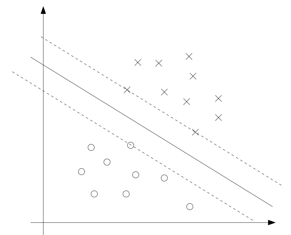
Therefore, by KKT dual complementary conditions, $\alpha_i >0$ only for the training examples that have functional margin exactly equal to 1.

The points with the smallest margins are the exactly the ones closest to the decision boundary. Thus, only three of the $\alpha_i$’s that corresponds to the three training example which has the smallest margins have non-zero at the optimal solution. These three points are called the support veectors

💡

The fact is that the number of support vectors can be much smaller than the size of the training set. (So, it is computationally efficient)

When we construct the Lagrangian for our optimization problem we have:

$$\mathcal L(w, b, \alpha) = \frac{1}{2}\|w\|^2 - \sum_{i - 1}^m \alpha_i[y^{(i)}(w^Tx^{(i)} + b) - 1]$$

Let’s find the dual form of the problem. To do so, we need to first minimize $\mathcal L(w, b,\alpha)$ with respect to $w$ and $b$, to get $\theta_\mathcal D$.

$$\nabla_w\mathcal L(w, b, \alpha) = w-\sum_{i = 1}^m \alpha_iy^{(i)}x^{(i)} = 0 \\\nabla_b\mathcal L(w, b, \alpha) = \sum_{i = 1}^m \alpha_iy^{(i)} = 0$$

This implies that

$$w = \sum_{i = 1}^m\alpha_iy^{(i)}x^{(i)}$$

By using these equations, we can reformulate the original Lagrangian as follows

$$\mathcal L(w, b,\alpha) =\sum_{i = 1}^m\alpha_i - \frac{1}{2}\sum_{i, j = 1}^my^{(i)}y^{(j)}\alpha_j(x^{(i)})^Tx^{(j)}$$

Therefore, we obtain the following dual optimization problem :

$$d^* = max_\alpha \theta_D(\alpha) = \max_{\alpha}\Big[\sum_{i = 1}^m\alpha_i - \frac{1}{2}\sum_{i, j = 1}^my^{(i)}y^{(j)}\alpha_j(x^{(i)})^Tx^{(j)}\Big] \\ \text{subject to }\alpha_i\ge0, i = 1,\dots, m \\ \text{and }\sum_{i = 1}^m\alpha_iy^{(i)} = 0$$

💡

The original optimization problem satisfy KKT condition because $f$ and $g_i$ are convex function and $g_i$ is feasible for all $i$. So, we can solve the original optimization via the dual optimization problem.

💡

Dual optimization has inner-product term. So by using this term, we can use kernel trick.

After we find $\alpha^*$, we can easily derive $w^*$ by using $w = \sum_{i = 1}^m\alpha_iy^{(i)}x^{(i)}$. In addition, we can also find $b^*$ by using following fact

$$\min_{y ' = 1}w^{*^T}x' + b^* = 1 \\ \max_{y ' = -1}w^{*^T}x' + b^* = -1$$

Suppose we’ve fit our model’s parameters to a training set, and now wish to make a prediction at a new point input $x$. We would then calculate $w^*x + b$, and predict $y = 1$ iff this quantity is bigger than zero. By using $w = \sum_{i = 1}^m\alpha_iy^{(i)}x^{(i)}$, we can derive

$$w^{*^T}x + b^* = \Big(\sum_{i = 1}^m\alpha_iy^{(i)}x^{(i)}\Big)^Tx + b^* \\ = \sum_{i = 1}^m\alpha_i^*y^{(i)}\langle x^{(i)}, x\rangle + b^*$$

Hence, if we’ve found the $\alpha_i$’s, in order to make a prediction, we have to calculate a quantity that depends only on the inner product between $x$ and the points in the training set. Moreover, we saw earlier that the $\alpha_i$’s will all be zero except for the support vectors . So we really need to find only the inner products between $x$ and the support vectors.

💡

By using Dual optimization problem, we can able to write the entire algorithm in terms of only inner products between input feature vectors. By using this fact, we can use kernel so that it can be able to efficiently learn in very high dimensional spaces.

Meaning of Basis function

A basis function is a function used to construct a particular function or set of functions as a linear combination of the basis function. Let $f$ is a function which is we wanted to find. We can construct this function as a linear combination of the basis function.

$$f(x) = \sum_{i = 0}^{L}\theta_i\phi_i(x) \\ =\theta^T\phi(x)$$

💡

Note : $\phi_1, \cdots, \phi_L$ is linearly independent

Since $\text{span}\{\phi_1, \cdots, \phi_L\}$ is isomorphic to $\R^L$, we can think

$$\phi : \R^d \to \R^L$$

So, we can think that

$$\phi(x) = Ax$$

And we want to take cost function to

$$\forall i \in [1, n], g(x_i|y_i, \theta) = \frac{1}{2}(y_i - f(x_i))^2 \\ = \frac{1}{2}(y_i - \theta^T\phi(x_i))^2$$

when we have $n$ data.

We want to find the optimal $\theta$ (i.e. we want to regard this function as a function of $\theta)$

$$\nabla_\theta g = -(y_i - \theta^T\phi(x_i))\phi(x_i)$$

Batch gradient descent

So, gradient descent for $\theta$ is following (Batch gradient descent case)

$$\theta := \theta -\alpha\sum_{i = 1}^n\nabla_\theta g(x_i) \\ =\theta + \alpha\sum_{i = 1}^n(y_i-\theta^T\phi(x_i))\phi(x_i)$$

Stochastic gradient descent

For i in range(1, n):

$$\theta := \theta -\alpha\nabla_\theta g(x_i) \\ \theta + \alpha(y_i-\theta^T\phi(x_i))\phi(x_i)$$

Conclusion

Using basis functions can help increase the dimensionality of the input space, which can make it easier to find decision boundaries or capture more complex relationships between the inputs and outputs.

Above example shows that input space is d-dimensional, however, output space is L-dimensional.

Kernel Trick

Actually, we can express $\theta$ as a linear combination of $\phi(x_1), \cdots, \phi(x_n)$ which are generated by input values.

💡

Note : We don’t know whether $\phi(x_1), \cdots, \phi(x_n)$ is independent. We just know that basis function is independent.

When we update the value of $\theta$ by using batch gradient descent twice, we can easily find that

$$\theta := \theta + \alpha \sum_{i = 1}^n(y^{(i)} - \theta^T\phi(x^{(i)}))\phi(x^{(i)}) \\ = \sum_{i = 1}^n\beta_i \phi(x^{(i)}) + \alpha \sum_{i = 1}^n(y^{(i)} - \theta^T\phi(x^{(i)}))\phi(x^{(i)}) \\ = \sum_{i = 1}^n \{\beta_i + \alpha (y^{(i)} - \theta^T\phi(x^{(i)}))\}\phi(x^{(i)})$$

Let $\beta_i := \beta_i + \alpha (y^{(i)} - \theta^T\phi(x^{(i)}))$, we can easily found that $\theta$ could be expressed by just linear combination of $\phi(x_1), \cdots, \phi(x_n)$.

💡

To do this, we initialize the parameter $\theta$ = 0

Since $\theta$ could be express by linear combination of $\phi(x_1), \cdots, \phi(x_n)$,

$$\beta_i := \beta_i + \alpha(y^{(i)} - \sum_{j = 1}^n\beta_j\phi(x^{(j)})^T\phi(x^{(i)})) \\ = \beta_i + \alpha(y^{(i)} - \sum_{j = 1}^n\beta_j \langle \phi(x^{(j)}), \phi(x^{(i)}) \rangle )$$

💡

Actually, we want to find the optimal value of $\theta$. But $\theta$ can be express by linear combination of $\phi(x_1), \cdots, \phi(x_n)$ with coefficient $\beta_1, \cdots, \beta_n$ respectively. So if we find optimal $\beta$, it is equivalent to find the optimal value of $\theta$.

So, from now on, we are focusing on finding an optimal value of $\beta$.

Why we have to do this procedure

1. $\langle \phi(x^{(j)}), \phi(x^{(i)}) \rangle$ can be pre-calculated for all pairs of i and j.

2. In addition, we don’t have to compute $\phi(x^{(i)})$ explicitly, when we try to calculate $\langle \phi(x^{(j)}), \phi(x^{(i)}) \rangle$

Regularization and the non-separable case

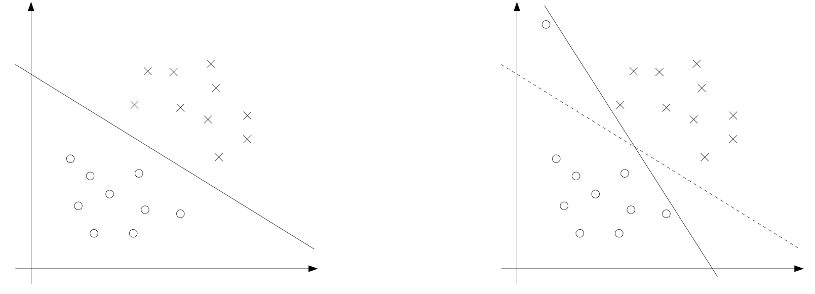
The derivation of the SVM as presented so far assumed that the data is linearly separable.However, we can’t guarantee that it always will be so. In addition, the original SVM approach is very sensitive to outliers.

The above figure shows that just one outlier changes the decision boundary dramatically. To make the algorithm work for non-linearly separable datasets as well as be less sensitive to outliers, we reformulate our optimization (using $\mathcal l_1$ regularization) as follows

$$\min_{w, b,\xi}\frac{1}{2}\|w\|^2 + C\sum_{i = 1}^m\xi_i\\ \text{subject to }y^{(i)}(w^Tx^{(i)} + b) \ge 1 - \xi_i, i = 1,\dots, m \\ \text{and }\xi_i\ge0, i = 1, \dots, m$$

💡

By doing so, the formula is permitted to have functional margin less than 1 and if an example has functional margin $1-\xi_i$, we would pay a cost of the objective function being increased by $C\xi_i$.

As before, we can form the Lagrangian:

$$\mathcal L(w, b,\xi, \alpha, r) = \frac{1}{2}w^Tw + C\sum_{i = 1}^m\xi_i - \sum_{i - 1}^m \alpha_i[y^{(i)}(w^Tx^{(i)} + b) - 1+\xi_i] - \sum_{i = 1}^mr_i\xi_i$$

After we calculate the dual form, we can derive

$$\max_\alpha \sum_{i = 1}^m\alpha_i - \frac{1}{2}\sum_{i, j = 1}^my^{(i)}y^{(j)}\alpha_i\alpha_j\langle x^{(i)}, x^{(j)}\rangle \\ \text{subject to }0\le\alpha_j\le C, i = 1, \dots, m \\ \text{and }\sum_{i = 1}^m\alpha_iy^{(i)} = 0$$