Computer Science/Machine learning
2. Review on Probability Theory
- -
728x90
반응형
Probability Space
Definition of Probability space
A probability space is defined by triplet
: Sample space
: -algebra on
:
Definition of Sample space
Set of all possible outcomes, where an outcome is the result of a single execution of the model
Definition of Event
Subsetof Sample space()
Definition of Field
A collection of subset of forms a field if following 3 conditions hold.
(It is equivalent to is a collection of events on )
-
-
- (closed under
finiteunion and intersection)
Definition of -field
A collection of subset of forms a -field if following 3 conditions hold.
(Almost same as the definition of Field except the 3rd condition)
-
-
- (closed under
countableunion and intersection)
Why we need to define -field
It requires to formally define the probability.
What is probability measure?
We say ()is a probability measure if satisfy 3 conditions.
-
-
- 채
Properties of probability
Joint probability
Marginal probability
Independence
Conditional probability
→ If A, and B are independent,
Law of total probability (a.k.a marginalization)
- is a partition of
💡
Marginalizing out unwanted data is a basic operation to process raw data
Countable additivity
For all countable collection of pairwise discoint events
Bayes theorem (very important in ML)
→ In ML, model typicall explains P(x|y)P(y) rather than P(y|x)

→ 정리할 것
What is Support?
First, we need to distinguish between the support of a random variable and the support of its distribution
The support of a random variable X
The support of a random variable X is the set of all possible values that can take on with non-zero probability.
- When X is a discrete r.v
The support is the set of
all possible valuesof
- When X is a continuous r.v with probability density function f(x)
The support is the set of all values of x for which f(x) is
non-zero
The support of a probability distribution
The support of a probability distribution is the set of all values of the random variable for which the probability density function is non-zero.
- When f(x) is discrete probability distribution
The support is the set of all values for which the probability mass function is non-zero
- When f(x) is continuous probability distribution
The support is the set of all values of x for which f(x) is non-zero.
Why we need to distinguish two concepts?
The support of a probability distribution can be different from the support of the random variable generated by that distribution.
For example, if X is generated by a uniform distribution over the interval (-1, 1), then its probability density function f(x) is:
In this case, f(x) has an infinite support, since it is non-zero over the interval (-1, 1) and zero elsewhere. However, X has a finite support, since it can only take on values in the interval (-1, 1). So in this case, the statement "X has a finite support" is true, even though f(x) has an infinite support.
Continuous Probability
→ a probability of a single point is always zero
→ the probabilities are measured over intervals
Bernoulli Distribution
Bernoulli distribution with parameter
Binomial Distribution
A binomial random variable can be interpreted as the sum of n independent Bernoulli random variables.
Beta Distribution
Beta distribution with parameters
Beta distribution is often used to model parameter p of bernoulli distribution
Beta distribution
In probability theory and statistics, the beta distribution is a family of continuous probability distributions defined on the interval [0, 1] in terms of two positive parameters, denoted by alpha (α) and beta (β), that appear as exponents of the variable and its complement to 1, respectively, and control the shape of the distribution.
 https://en.wikipedia.org/wiki/Beta_distribution
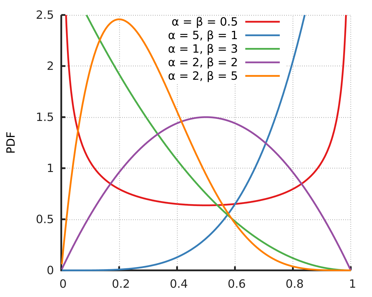
Gaussian Distribution
Central Limit Theorem
저번 학기 확률통계 한번 더 읽어볼 것
n → 로 갈 때
Multivariate Gaussian PDF
Multivariate normal distribution
In probability theory and statistics, the multivariate normal distribution, multivariate Gaussian distribution, or joint normal distribution is a generalization of the one-dimensional (univariate) normal distribution to higher dimensions. One definition is that a random vector is said to be k-variate normally distributed if every linear combination of its k components has a univariate normal distribution. Its importance derives mainly from the multivariate central limit theorem. The multivariate normal distribution is often used to describe, at least approximately, any set of (possibly) correlated real-valued random variables each of which clusters around a mean value.
https://en.wikipedia.org/wiki/Multivariate_normal_distribution
반응형
Contents
소중한 공감 감사합니다