3. Linear Regression

2_Linear_Regression.pdf

Basic Notation

$x^{(i)}$ : input variables

$y^{(i)}$ : Output variables (label)

$(x^{(i)}. y^{(i)})$ : A training example

$\{(x^{(i)},y^{(i)})|i = i, \cdots, n\}$ : A training set

$\mathcal X$ : The space of input values

$\mathcal Y$ : The space of output values

Goal of Supervised Learning

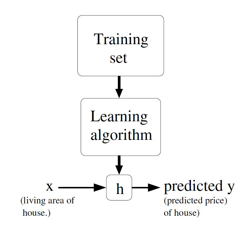
The goal of supervised learning is to learn a function h : x → y

1. Regression : the target value is continuous

2. Classification : the target variable can take only small number of discrete values.

Linear Regression

Linear combination of input features.

Goal : Find the parameters that parameterize the space of linear functions mapping from $\mathcal X \to \mathcal Y$.

$$h(x) = \sum_{i = 0}^d \theta_ix_i = \theta^Tx : \text{inner product}$$

Cost function

$$J(\theta) = \frac{1}{2}\sum_{i = 1}^n (h_\theta(x^{(i)}-y^{(i)})^2$$

Less cost function value man that better function

How to find the optimal theta

1. Iterative Updates of theta : gradient descent algorithm

2. Closed form solution for theta

Iterative Updates

updates the value of theta with the learning rate alpha

What does it imply?

Error가 크면 theat가 변화하는 정도가 큼

Batch gradient descent

배치 단위로 theta를 업데이트

It looks at every example in the entire training set on every step

Stochastic gradient descent

The parameters are updated according to the gradient of the error with respect to that single training example only

Stochastic gradient descent

Stochastic gradient descent is an iterative method for optimizing an objective function with suitable smoothness properties. It can be regarded as a stochastic approximation of gradient descent optimization, since it replaces the actual gradient by an estimate thereof. Especially in high-dimensional optimization problems this reduces the very high computational burden, achieving faster iterations in exchange for a lower convergence rate.

https://en.wikipedia.org/wiki/Stochastic_gradient_descent

(차이 집에가서 정확히 정리 훈련 당시와 test당시의 상황이 다름)

→ Really scalable, messy dataset을 가진 경우 stochastic gradient descenet를 사용하는 것이 좋음.

Closed form solution

Minimize the cost explicitly without relying on an iterative algorithm?

→ 미분하고 해당 값이 0

J(\theta) 는 scalar

We are implicitly assumption $X^TX$ is invertible

Not inverted case

1. number of linearly independent examples is fewer than the number of features

2. the features are not linear independent with each other.

Pros

Directly compute/estimate theat prarmeter without iterating update.

Cons

Inverse matrix operation is really expensive.

In addition it is no garantee for inverse matrix exist.

Probabilistic interpretation

Is really the least-square cost function. J a reasonable choice?

epsilon : error (where iid from Normal dist)

$y^{(i)} - \theta^Tx^{(i)} = \epsilon^{(i)}$ 를 통해서 gaussian distribution으로 돌림

Likelihood function

“How likely” the data are observed given the model paramters

: Theta 가 주어졌다고 했을 때, 얼마나 x로부터 y가 나올 것인지를 예측하는 것 (해당 확률이 높을 수록 theta가 좋다는 의미)

→ Likelihood가 높게끔 하는 theta를 찾겠다는 것이 목표

Basis Function

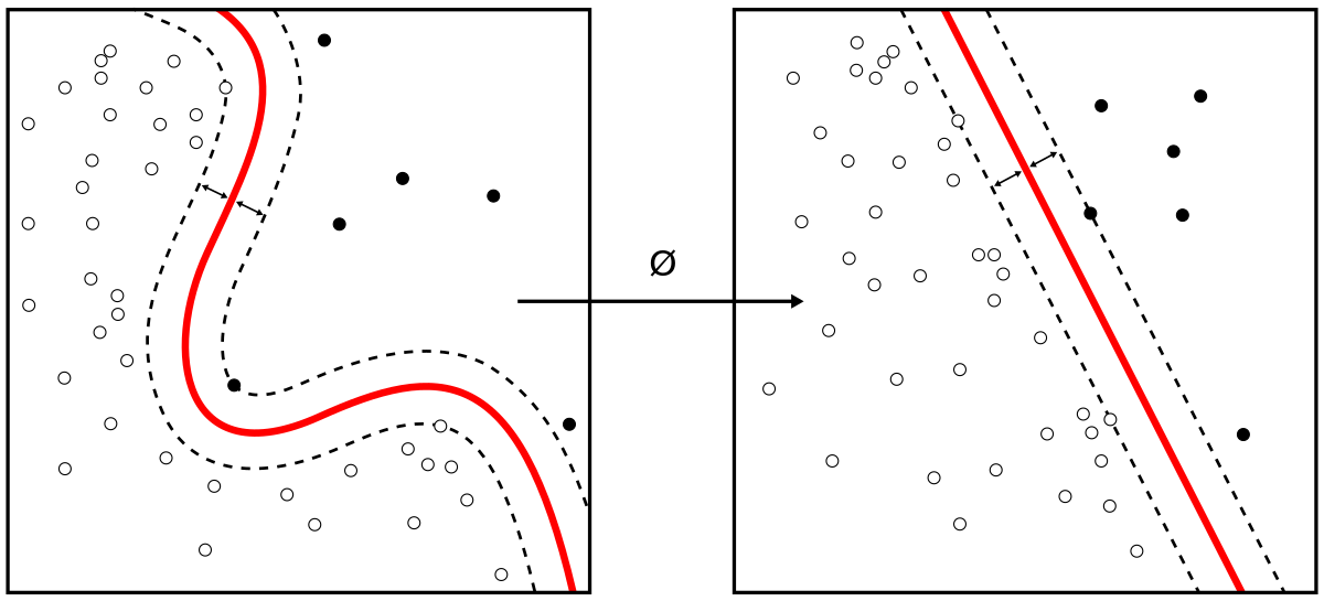
Basis를 linear 함수로 제한시키는 것이 아니라 vector space를 이용해서 확장시키는 것.

1. Polynomial basis

2. Gaussian basis

   Exponential Functions build Basis for Vector Space

   Let $V$ be a subspace of the $R$-Vectorspace of all differentiable functions defined by $V := span\{(t-34)e^t, (6t+1)e^t + e^{2t}, e^{2t}, e^t\}$. I do not know how to start with finding a basis for

   https://math.stackexchange.com/questions/4520296/exponential-functions-build-basis-for-vector-space

   

Underfitting and Overfitting

When the number of parameters is small, an ùnerfitting issue can occur

In contrary , when the number the parameters is large, an overfitting issue can occur

How can we handle the overfitting problem?

Non-paramtetric algorithm

Locally weighted linear regression, It is well known for handling overfitting problem

Regularized paramters

It uses an additional regularizer term to decrease magnitude of parameters

Locally weighted linear regression

1. 새로운 paramter W가 등장(각 training example에 대해서 각각 존재)

   만약 w가 굉장히 크면, error를 작게 만들기 힘듬. 반대로 작으면 해당 데이터셋을 무시하게 됨.

   Standar choice for weights with the bandwidth paramter $\tau$

   

   Note that the weights depend on a particular point x at which we are trying to evaluate x

   (찾으려는 x와 가깝게 존재하는 것을 크게 보정한다.)

   Ridge Regression

   Overfitting issues are usally observed when the maginitude of paramters is alrge

   → theta가 크면 오버피팅 이슈가 일어날 가능성이 높음

   따라서, theta의 magnitude를 줄이는 regularator를 줌

   $\theta^T\theta$ : regularizor

   이를 통해 generalization을 늘림

   $\lambda : hypterparameter$ (인간의 경험으로 선택)

   정규방정식을 통해 계산을 하면

   $\lambda I$ 가 inverse쪽에 새로 추가된다는 점에서 차이가 있음.

   만약 $\lambda$가 굉장히 작은 경우 : overfitting

   반대의 경우에는 underfitting

Maximum A posteriori

세타도 분포를 따른다고 가정하고 모델링(이전까지는 세타가 고정된 값이라고 가정)

→ 즉, optimal 세타를 찾는 것이 목표

Likelihood : 주어진 세타에 대한

주어진 데이터에 대해서 세타가 나올 확률이 얼마나 되는지 (이걸 베이즈 정리로)

세타 역시 dist를 따른다고 하면 prior까지 곱한 것이 최대가 되게끔!

각각의 gaussian 공식을 사용해서 최대가 되게끔하는 세타를 구하면 됨

여기에서 시그마를 줄인다는 것을 람다를 키운다는 것과 같다는 ridge regression의 결론과 연관지을 수 있다.

정리

$p(x|y, \theta)$ is easily compute than $p(y|x, \theta)$

$p(x|y,\theta)$ involves modeling the relationship between the input variables $x$ and output variables $y$. This relationship may be more straightforward to model because we have direct control over the input.

In contrary, $p(y|x, \theta)$ requires us to understand the complex interactions between the input and output variables. Additionally, the output variable $y$ may have a more complex distribution than the input variable $x$, making it harder to model.

Procedure of probabilistic model

💡

Remember that what we want to know is the distribution of $p(y|x, \theta)$

1. Define the conditional probability distribution $p(y|x,\theta)$

   For example, suppose we have a dataset of student exam scores, where each student has taken two exams: Exam 1($x_1$) and Exam 2($x_2$), and each student is either admitted $(y = 1$) or not admitted $(y = 0$) to a university.

   We simply define the conditional probability distribution

   $$p(y = 1|x, \theta) = \frac{1}{1 + e^{-\theta_0 + x_1\theta_1 + x_2 \theta_2}}$$

2. Find the optimal value of $\theta$ by using MLE (Assume that i.i.d)

   $$\argmax_\theta\mathcal L(\theta;D) := \argmax_\theta \prod_{i = 1}^n p(y_i|x_i, \theta)$$

   where $D = \{(x_1, y_1), \cdots, (x_n, y_n)\}$ is the training dataset

   Take the logarithm of both sides

   $$\argmax_\theta log\mathcal L(\theta; D) = \argmax_\theta \sum_{i = 1}^n log(p(y_i|x_i, \theta))$$

What about the non-supervised learning? How can we define likelihood function?

Let's consider a clustering problem where we want to group a set of data points into different clusters. We can use a probabilistic model such as the Gaussian mixture model (GMM) to do this.

In the GMM, we assume that the data points come from a mixture of Gaussian distributions, where each cluster is characterized by a mean and covariance matrix. The goal is to estimate the parameters of the model that best fit the data.

The likelihood function for the GMM is defined as:

$p(X | \theta) = \prod_{i=1}^{N} \sum_{k=1}^{K} \pi_k \mathcal{N}(x_i | \mu_k, \Sigma_k)$

where X is the dataset, N is the number of data points, K is the number of clusters, $\theta = (\pi_1, ..., \pi_K, \mu_1, ..., \mu_K, \Sigma_1, ..., \Sigma_K)$ are the parameters of the model, $\pi_k$ is the mixing coefficient for the k-th cluster (i.e., the prior probability of a data point belonging to the k-th cluster), and $\mathcal{N}(x_i | \mu_k, \Sigma_k)$ is the probability density function of a Gaussian distribution with mean \mu_k and covariance matrix $\Sigma_k$ evaluated at data point $x_i$.

The log-likelihood function is then:

$$log p(X | \theta) = \sum_{i=1}^{N} log \bigg( \sum_{k=1}^{K} \pi_k \mathcal{N}(x_i | \mu_k, \Sigma_k) \bigg)$$

The goal in this case is to maximize the log-likelihood function with respect to the parameters $\theta$, which can be done using an algorithm such as the expectation-maximization (EM) algorithm.

GMM(Gaussian Mixture Model,가우시안 혼합모델) 원리

개인공부용 블로그로 이곳의 내용에 개인적으로 추가정리하였다. 가우시안 분포는 데이터를 분석하는 데 있어서 중요한 여러 성질을 가지고 있지만, 실제 데이터셋을 모델링 하는데에는 한계가 있다.(어떻게 모든 데이터가 종모양분포를 띄겠나...) 그래서 나오게 된 것이 Gaussian Mixture Model(GMM)인데, 여기서 mixture model이라는 것의 뜻은 기본분포를 선형결합해서 만든 분포라는 뜻이다. 그러므로 GMM은 가우시안분포를 선형결합하여 만들어진 분포를 뜻한다. (이런식으로 모델을 딱 가정해버리면 모델에 들어가는 파라미터를 찾는 식으로 밀도를 추정하게 된다. 만약 모델을 가정하지 않는다면, non-parametric하게 밀도를 추정하게 된다. ex.커널밀도추정) 예를들어 위의 오른쪽 그림과..

https://sanghyu.tistory.com/16