6. Bayesian Networks

Definition

Bayesian networks are networks of random variables

→ Each variable is associated with a node in the network

If we know of the existence of conditional independencies between variables we can simplify the network by removing edges

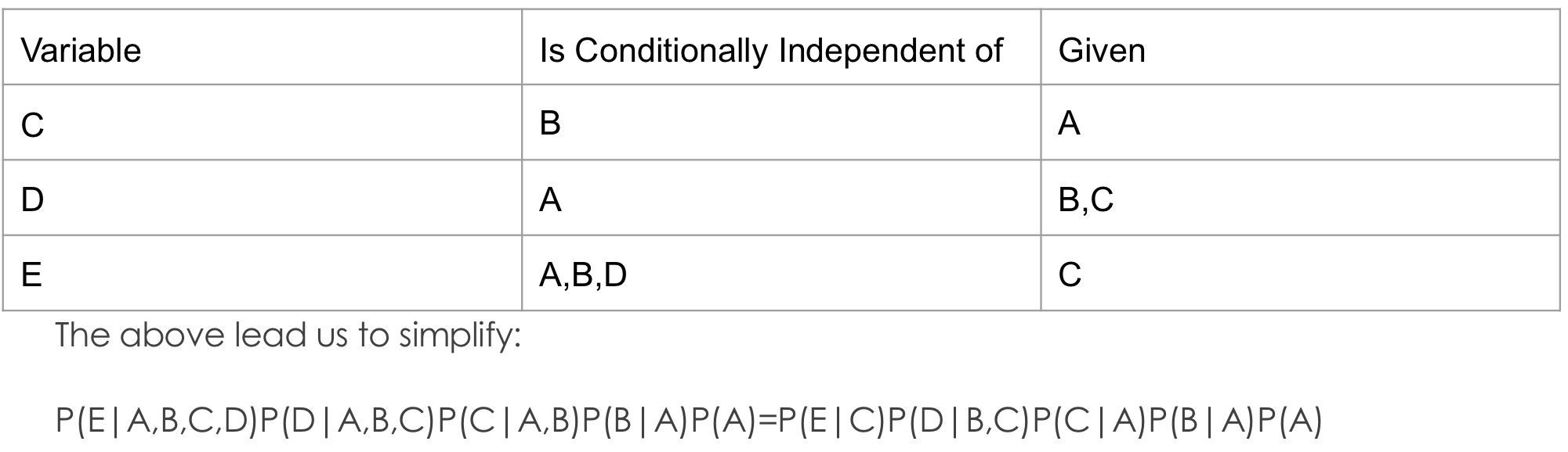
This leads to the simplified network

💡

여기에서 연결된 edge가 없으면 conditional independence를 함축한다.

Causal Networks

While correlation (association) between variables is an important observation in data analysis, it does not provide evidence for establishing causal relationships.

→ Correlation doesn’t imply causation

Dynamic Bayesian Networks

Bayesian networks can be dynamic . In fact, a HMM(Hidden Markov model) is a very simple dynamic Bayesian network.

Fitting a Bayesian Network to Data

We could model this with any sort of statistical model we like.

→ 수업에서는 categorical distribution 을 사용함

💡

추가적으로 categorical distribution으로 fitting할 때 label smoothing을 처리하기 위해 1을 base로 깔고 시작한다는 점을 유념해야 한다.

Example

Markov Chain Monte Carlo (MCMC) Sampling

General Idea

We can estimate the probability distributions of any set of unknown variables given any set of observed variables. However, generally approximate inference is performed using sampling.

• Basic Idea
  1. Assume we want to estimate the distribution P
  2. Set up a Markov chain whose long run distribution is P
  3. Evolve the Markov chain to generate samples

     → As the number of samples approaches infinity, the sample distribution approaches P

  4. Use these samples to estimate P

• Approach
  1. Gibbs Sampler
  2. Metropolis
  3. Metropolis within Gibbs

💡

MCMC는 높은 차원의 확률 분포로부터 직접 샘플링하기 어려울 때 유용하게 사용된다.

• Aim : Given a set of known (or assumed) variables, E , estimate the probability distributions of the remaining unknown variables, U

• Algorithm
  1. Initialization
     1. Perform a topological sort on the graph
     2. Set all variables in E to their known/assumed values
     3. Randomly assign values to each variables in U

     💡

     Topological sort를 하는 이유는 해당 정렬을 하게 되면 한 변수가 다른 변수에 의존하는 경우 그 의존하는 변수가 먼저 오게 된다는 것을 반드시 보장할 수 있기 때문이다.

  2. Generate n samples (done differently in each algorithm)
  3. Use these samples to estimate desired distributions

We can’t know that a run of MCMC samples has succeeded in converging to the desired distribution

1. Common to perform multiple runs, from different initial origins

2. If these converges with each other, we hope all have converged with the underlying distribution

   → But degenerate cases is possible : 즉 대상 분포가 아닌 다른 어떤 분포에 수렴하거나 chain 중 일부만 target distribution에 수렴하지 않을 수 있다는 의미이다.

Gibbs Sampling

The basic idea of Gibbs Sampling is to sequentially update each variable according to its conditional probability distribution, given the current values of all other variables.

Here are the basic steps in the Gibbs Sampling algorithm:

1. Initialization: Set initial values for all variables randomly.

2. Iteration: At each iteration step, select one variable and update it while keeping all other variables fixed. This variable is updated according to its conditional probability distribution given the current values of all other variables.

3. Convergence: After enough iterations, the generated samples will approximate the target multivariate probability distribution.

Gibbs Sampling allows you to draw samples from complex multivariate distributions if you only know each variable's conditional distributions given others' current values - making it widely used in fields like Bayesian statistics and machine learning.

Note : The Markov blanket of a node in a Bayesian network consists of the node’s parents, its children, and co-parents of its children.

💡

Gibbs Sampling에서 가장 중요한 것은 한번에 한 변수를 고르고 나머지를 고정시킨 상태로 update를 진행한다는 점이다. 반면 Metropolis의 경우 한번에 업데이트를 진행하게 된다.

Metropolis

The Metropolis algorithm is a type of Markov Chain Monte Carlo method used for sampling for complex probability distributions

Here’s the basic working principle of the Metropolis algorithm:

1. Initialization : Choose an arbitrary starting point

2. Proposal : From you current position, propose a new point using a proposal distribution . This proposal distribution is often something symmetric like a normal distribution, but it doesn’t have to be

3. Acceptance/Rejection : Calculate the probability values of the new and current points under your target probability distribution and decide whether to accept or reject the new point.

   → If the new point has higher probability than your current one, you always accept it. if not, you accept it with a probability proportional to the ratio of their probabilities under your target distribution. ($p : \min(1, p_{new}/p_{old})$)

4. Iteration : Repeat this process many times to generate a Markov chain

After enough time has passed, this generated Markov chain will follow your target probability distribution. One reason why the Metropolis algorithm is widely used is its flexibility in application. It can be applied even when your objective function isn’t normalized or directly computable over all space.

• Q : What is the different between Metropolis Algorithm and Gibbs Sampling

  Both the Metropolis algorithm (and its generalized version, the Metropolis-Hastings algorithm) and the Gibbs sampling algorithm are types of Markov Chain Monte Carlo (MCMC) methods that make use of information about conditional distributions. However, they do so in different ways.

  1. Metropolis-Hastings Algorithm: This algorithm does not explicitly require knowledge of conditional distributions. Rather, it needs to know the target distribution up to a constant of proportionality. Given a current state in the Markov chain, it proposes a new state according to some proposal distribution and then decides whether to accept this new state or stay in the current state based on an acceptance probability that involves ratios of densities from the target distribution.

  2. Gibbs Sampling: This is a special case of Metropolis-Hastings where we specifically use full conditional distributions for proposing new states in our Markov chain. In Gibbs sampling, we cycle through each dimension (or variable) of our multivariate distribution one at a time and sample from its full conditional distribution while keeping all other dimensions fixed at their current values.

  So while both algorithms utilize information about distributions associated with our target multivariate distribution, they do so differently: Metropolis-Hastings can operate with just knowledge about unnormalized densities from our target distribution while Gibbs sampling requires explicit knowledge about full conditional distributions.

Note : Care must be taken with the proposal function such that a reasonable acceptance rate is maintained. This can be difficult with a large number of variables.

→ In such a case, Metropolis in Gibbs may be a better alternative.

Metropolis in Gibbs

It basically uses a Metropolis step within a Gibbs sampler. This is sometimes necessary when it’s difficult or impossible to sample directly from the full conditional distributions required for a pure Gibbs Sampler.

Here’s the basic working principle of the Metropolis in Gibbs algorithm:

1. Initialization : Choose an initial state for all variables in your model

2. Iteration : For each iteration of the algorithm, do the following
   1. Fix the values of all other variables at their current states
   2. Sample a candidate value for the current variable from its proposal distribution
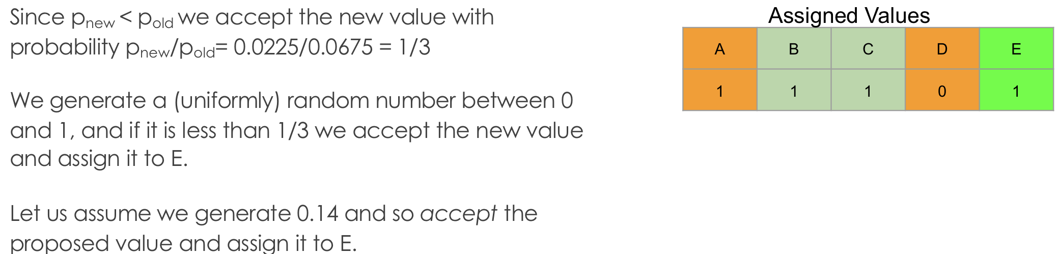
   3. Calculate an acceptance probability for old variable and new variable
   4. Assign the value with probability $p : \min(1, p_{new}/p_{old})$. Otherwise it remains assigned the old value

3. Record the assigned values of all variables as a sample

It is often easier to maintain a reasonable acceptance rate in Metropolis in Gibbs than in the pure Metropolis algorithm.

💡

acceptance rate는 제안된 새로운 상태를 얼마나 자주 받아들일지에 대한 비율이다. 해당 값이 너무 높다면 공간을 충분히 탐색하지 못하는 문제가 있고, 너무 낮으면 MCMC chain이 많은 단계에서 움직임 없이 현재 위치에 머무르게 되며 이에 따라 수렴까지 오랜 시간이 걸릴 수 있게 된다는 문제점이 있다.

💡

Metropolis algorithm은 전체 변수 공간에서 sampling을 진행하므로 적절한 proposal distribution을 선택하는 것이 매우 중요하다. 그렇지 않으면 acceptance rate가 떨어지게 된다. 반면 Metropolis in Gibbs의 경우에는 한번에 하나의 변수만 update하기 때문에 일반적으로 개별 변수의 conditional distribution이 잘 정의되어 있는 경우 합리적인 acceptance rate를 유지하는 것이 쉽다.

The price of this is that all individual steps are linear on the unknown variables, and so sometimes the Metropolis in Gibbs random walk will have difficulty crossing from on area of high probability to another. This can be a problem if the distribution being estimated is multimodal (more than one peak/mode)

💡

알려지지 않은 variable에 대해서 선형적이라고 가정하고 있다는 점이 문제가 될 수 있다는 것이다.

💡

Metropolis와 달리 Metropolis in Gibbs가 가지는 가장 큰 차이는 변수를 개별적으로 순차적으로 업데이트 한다는 것이다.

💡

기본적인 Metropolis algorithm은 전체 변수 공간에서 새로운 상태를 제안하고, 이를 수용할지 여부를 결정한다. 따라서 높은 probability density 영역 사이의 골짜기를 건너뛰는 것이 가능하다. 하지만, Metropolis in Gibbs는 각 단계에서 하나의 차원만 고려하므로, 각 차원 간에 복잡한 상호작용이 있는 경우나 분포가 multimodal인 경우에는 효율성이 떨어질 수 있다.

Example

Burn period

Since we arbitrarily assign initial value, initial samples are often biased. It is best to discard the first n samples. This is called the burn period

1. This bias will eventually be overcome. But if we don’t have a burn period, it requires more sample

2. You should always use a burn period

Thinning

Sampling is most efficient if the samples are uncorrelated. Since MCMC samples are very correlated, so we want to reduce its correlation by only keeping every 1 in n samples. This is called thinning

1. Thinning is useful only if the improvement obtained by somewhat de-correlating the samples outweights the improvement we would have got from working with more samples

2. Therefore, thinning is optional

Where is the Markov Chain?

The states are the samples, with the initial state the initial assignment of values

The transition matrix is implicitly determined by the conditional by the conditional distributions and the process involved in generating a new sample/state

💡

Markov chain은 sample 간의 의존성을 의미한다. 즉 각 sample은 이전 sample에 기반해서 생성되며 이러한 방식으로 Markov chain이 구축된다. 이러한 chain을 통해 원하는 target distribution으로 converge하는 것이 MCMC의 목표이다.

Intervention Analysis using Causal Networks

We intervene in a system when we force a variable to take a particular value.

Note this it not the same as estimating the effect of finding that the variable takes a value, since the latter tells us information about the causes of that variable.

If C is found to take a value, this tells us something not only about D and E but also about A.

But if we force C to take a value, this tells us nothing about A

Therefore, we can estimate the effects of intervention by removing all edges into forced variables, an then performing inference as usual.

💡

But it can only be done with causal networks