5. Markov Chains

Markov Chains

Markov Chains appear all over computer science, mathematics and AI. Just some of the applications

• Biology : birth death process, disease spreading

• Biology : DNA/RNA/Protein sequence analysis

• Speech recognition

• Control theory, filtering

💡

LLM(Large Language Model)의 경우 Markov Chain의 아이디어를 많이 차용하였다. 지금은 Deep learning algorithm으로 대체되기는 하였다.

Representing Markov Chain

• Markov chain과 Markov process와의 차이점이 무엇인가?

  일반적으로 Markov property를 만족하는 것을 Markov process라고 하고, 이 중 discrete한 경우를 Markov chain이라고 많이 부른다. 사실 2개의 용어를 크게 섞어써도 무방하기는 하다.

Assumption

• The system is in one of a number of states : $S_i$

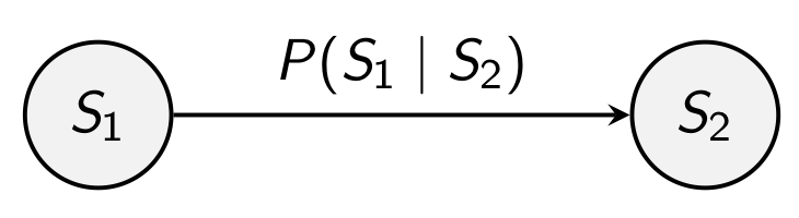
• For each pair of states $S_i$ and $S_j$, we have some probability $p_{i,j} = P(S_i|S_j)$ of going from state $S_i$ to $S_j$

• The probability only depends on a finite number of previous states

💡

즉 state들이 시간에 따라 변화하되, 그 확률은 이전 state에 의해서만 영향을 받는다고 가정하는 것이다.

예를 들어 날씨 예보 모델에서 하루하루의 날씨를 Markov chain으로 모델링한다면, '오늘'의 날씨는 '어제'의 날씨에만 의존하고 '그제'나 그 이전의 날씨는 고려하지 않는 것이다.

이러한 성질을 Markov property 혹은 memoryless 라고 불린다.

💡

Memoryless 성질은 특히 지수 분포(Exponential distribution)나 기하 분포(Geometric distribution)와 같은 확률 분포에서 잘 나타나며, 이들 분포는 자연과학이나 공학 등 여러 분야에서 발생하는 사건들을 모델링하는 데 널리 사용된다. 즉 현재의 state만으로 바로 다음 state의 확률을 예측할 수 있으므로 memoryless라고 하는 것이다.

따라서 우리는 system을 sequence of state 로 기술할 수 있게 된다.

$$S_0,S_1,\dots, S_n$$

💡

따라서 Markov chain으로 모델링하고자 하는 경우에는 state 를 정의하는 것이 굉장히 중요하다. 즉 주어진 문제나 데이터에 가장 적합한 방식으로 state를 잘 정의하는 것은 Markov Chain 모델링에서 중요한 과제이다.

Questions you can ask of Markov Models

1. Given probabilities what is the most likely sequence of states?

2. If I let the system run for a long time, what is the probability distribution of the states that I will end up in? What is the most likely state I will end up in?

3. Given a sequence of states, how likely is that sequence based on our model?

4. Can I estimate transition probabilities from the data?

5. Divide states into observable and hidden states. Given a sequence of observed states, what is the most likely sequence of hidden states that give you the observed states?

   💡

   이를 hidden Markov model이라고 한다.

Example - Rain or no Rain

• Two states $S = 0$ sunny, and $R = 1$ raining

• Initial probability distribution

  $$S_0 = (0.5, 0.5)$$

  50% chance of sunny, 50% chance of rain.

• We need four numbers $p(S|R), p(S|S), p(R|R), p(R|S)$

  $$\begin{bmatrix} p(S|S) & p(R|S) \\ p(S|R) & p(R|R)\end{bmatrix} = \begin{bmatrix} 0.8 & 0.2 \\ 0.4 & 0.6\end{bmatrix}$$

  💡

  transition probability를 matrix 형태로 표현한 것이다. 행렬 형태로 표현하면 수학적으로 계산을 좀 더 간편하게 할 수 있다. (이러한 행렬을 transition matrix 라고 한다.)

  💡

  앞에서 언급한 것처럼 system 자체를 state들의 sequence로 바라보겠다는 것인데, 해당 state들의 시간의 따른 변화에 대한 distribution 정보를 담고 있는 행렬이라고 생각해주면 된다.

After one day, what is the probability that it is sunny?

$$p(S_0)p(S_1|S_0) + p(R_0)p(S_1|R_0) = 0.5\cdot0.8 + 0.5 \cdot0.2$$

After one day, what is the probability that it is rainy?

$$p(S_0)p(R_1|S_0) + p(R_0)p(R_1|R_0) = 0.5\cdot0.4 + 0.5 \cdot0.6$$

💡

각 사건은 독립적인 사건이므로 쉽게 저렇게 나타낼 수 있다.

Therefore, we can interpret this result as

$$\begin{bmatrix}p(S_1) & p(R_1)\end{bmatrix} = \begin{bmatrix}p(S_0) & p(R_0)\end{bmatrix} \begin{bmatrix} p(S|S) & p(R|S) \\ p(S|R) & p(R|R)\end{bmatrix}$$

General Setting

Given $n$ states $(1, \dots, n)$, we have a $n$ by $n$ matrix $T$

$$\begin{bmatrix} p(1|1) & p(2|1) &\cdots &p(n|1) \\ p(1|2) & p(2|2) & \cdots &p(n|2) \\ \vdots & \vdots & \vdots & \vdots \\ p(1|n) & \cdots & \cdots & p(n|n)\end{bmatrix}$$

Given the initial distribution of states $S_0$ then after $n$ steps we end up in the distribution:

$$S_0T^n$$

💡

위의 예시의 경우에는 시간이 지남에 따라서 transition probability가 고정이라는 전제가 들어가 있다. 이때, 시간이 변함에 따라 transition probability가 변하지 않는 경우 homogeneous Markov chain 이라고 하고, 변하는 경우에는 non-homogeneous Markov chain이라고 부른다.

💡

이러한 과정을 무한번 반복한다고 해서 해당 system이 stationary distribution 으로 간다는 보장을 반드시 할 수 있는 것은 아니다. Convergence 여부는 따로 수학적으로 증명해주어야 한다.

Sampling from a Markov Chain

Useful for simulation

• Sample the initial state, randomly pick a state with the required probabilities

• Calculate the new state probabilities and sample again with the required probabilities

💡

이를 Monte Carlo Markov Chain (MCMC)라고 부른다. 이를 통해서 복잡한 확률 분포로부터 샘플을 추출할 수 있게 된다. 충분한 시간 동안 실행된 후 생성된 sample들은 원하는 target distribution으로부터 추출된 것처럼 간주할 수 있다.

Example

Two states $A$ and $B$ with probability distribution

$$(A = 0.65, B = 0.35)$$

and transition matrix

$$\begin{bmatrix} 0.3 & 0.7 \\ 0.5 & 0.5\end{bmatrix}$$

Sampling means that you pick $A$ or $B$ you have a $65$% chance of picking A

💡

즉, 초기 distribution을 기반으로 sampling을 하고 state를 고정시키겠다는 의미이다.

Suppose you pick $A$, this gives that state vector

$$(1, 0)$$

Calculate

$$\begin{bmatrix}1 &0\end{bmatrix} \begin{bmatrix}0.3 & 0.7 \\ 0.5 & 0.5\end{bmatrix} = \begin{bmatrix}0.3 & 0.7\end{bmatrix}$$

Then sample state $A$ and $B$ with probabilities 0.3 and 0.7

💡

즉, initial distribution을 업데이트한 효과를 가져온다. 이를 통해서 target distribution을 향해 수렴하게 된다.

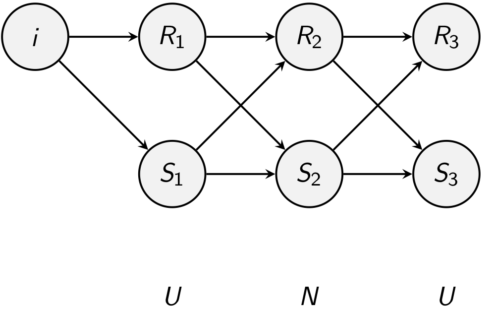
Hidden Markov Models

이전까지의 Markov model의 경우에는 observe 할 수 있는 state만을 다루었다. 반면 Hidden Markov Model의 경우에는 관찰할 수 없는 state들이 Markov property를 가지고 이러한 state가 observation에 영향을 주는 system을 다룬다.

💡

주의해야할 점은 observation이 Markov property를 가지는 것이 아니고, state 가 Markov property를 가지는 것이다.

Applications

• Speech recognition : You observe the sound (observation), and the hidden state is what word is being spoken

• Error correcting codes : You observe a noisy bit-stream (observation), and you want to infer the sent message (hidden state)

• Language processing : Given a sentence “The band goes whoop” work out the probability that “whoop” is an adverb or a noun (find hidden state) from it place in the sentence (observation)

• Biological sequence analysis : Genetic sequence have lots of codes, start and stop sequences, protein codes, etc. You observe the raw sequence AGTAGAATAA (observation) and you want to know what it is doing (hidden state).

Example

Divide the world up into states (Raining, $R = 0$, and Sunny $S = 1$) and observations (if my mother takes my Umbrella, $U = 1$, and not takes my Umbrella, $N = 0$)

💡

즉, hidden state는 sunny, raining이고 observation은 우산을 챙겨준 것의 여부이다. 즉 observation을 통해서 hidden state를 추정해야하는 상황이다.

As before, initial probability distribution is

$$S_0 = \begin{bmatrix} p(S) & p(R)\end{bmatrix}$$

Again we have a transition matrix for the states:

$$\begin{bmatrix} p(S|S) & p(R|S) \\ p(S|R) & p(R|R)\end{bmatrix}$$

Unlike before we need to know the probabilities that an umbrella will be used or not

$$\begin{bmatrix} p(N|S) & p(U|S) \\ p(N|R) & p(U|R)\end{bmatrix}$$

💡

직접적으로 관찰가능한 것은 우산을 챙겨준지 여부이다. 따라서 이를 바탕으로 하는 probability도 고려해야 한다. 또한 위 상황에서 observation은 current hidden state에만 의존한다.

Suppose I observe for three days and see $U, N, U$. What is the probability of this sequence?

💡

일반적인 Markov Chain과 달리 state를 직접 관찰할 수 없다는 점이 hidden Markov Chain의 가장 큰 특징이다.

If I knew that the hidden states on those three days were $R, S, R$ then I can use the conditional probabilities

$$p(U, N, U|R, S, R) = p(U|R)p(N|S)p(U|R)$$

💡

기본적으로 observation을 가정하고 hidden state를 바라보는게 더 자연스럽다. 이런 느낌으로 해당 식을 바라보면 직관적으로 이해할 수 있다.

For three days there are 8 possible sequence of internal hidden states

$$p(U, N, U|RRR) \\ p(U, N, U|RRS) \\ \vdots \\ p(U, N, U|SSS)$$

But you have to note that each term are not equally likely. So we have to weight each item by multiplying the probability that observation occurs

$$p(U, N, U|RRR)\cdot p(RRR) \\ p(U, N, U|RRS)\cdot p(RRS) \\ \vdots \\ p(U, N, U|SSS)\cdot p(SSS)$$

But this approach is impractical. So we are going to use dynamic programming instead

💡

잘 생각해보면 중복되는 계산이 생각보다 많다. 따라서 dynamic programming을 통해 중복된 계산을 최대한 하지 않겠다는 의미이다.

By Bayes’ theorem

$$p(R_1|U) = \frac{p(U|R_1)p(R_1)}{p(U)} \\ p(S_1|U) = \frac{p(U|S_1)p(S_1)}{p(U)}$$

But we have the same factor $p(U)$ in each term. So we just calculate the numerator and scale it.

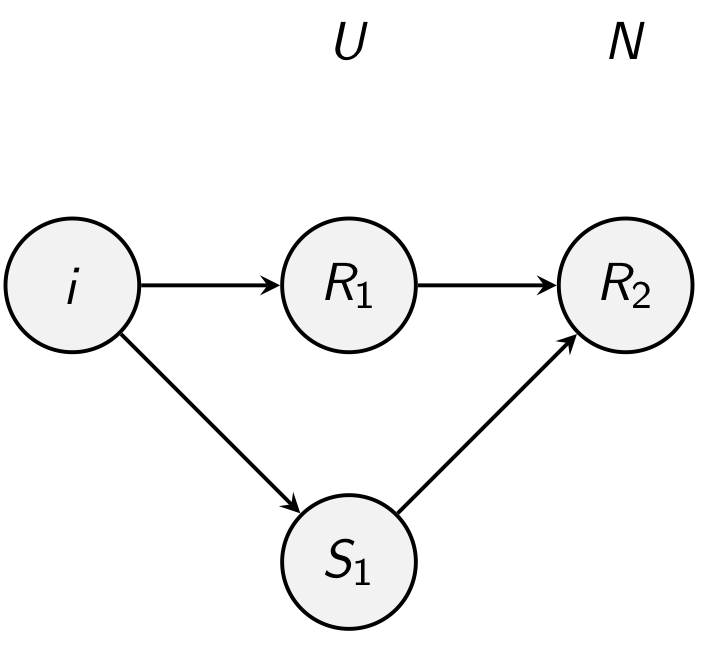
Then how do we calculate $p(R_2 |UN)$. The Markov assumption is that the current state only depends on the previous state. We can get $R_2$ from $R_1$ or $S_1$, and we have already calculated those probabilities

$$p(R_2|UN)\propto p(UN|R_2)p(R_2)$$

💡

Posterior랑 느낌이 거의 유사하다. 어차피 denominator는 나중에 rescaling만 하면 되므로 크게 고려하지 않아도 된다.

Since, $U$ is only related to $R_2$

$$p(R_2|UN)\propto p(U|R_2)p(R_2)$$

💡

$p(UN|R_2) = p(U|R_2)$임을 주의해야 한다. Hidden Markov Chain에서 특정 시점 t에서의 observation은 특정 시점 t에서의 hidden state값에만 의존한다. 따라서 N을 무시하는 것이다.

In addition

$$\begin{align}p(R_2) &= p(R_2|R_1)p(R_1|N)p(N) + p(R_2|S_1)p(S_1|U_1)p(N) \\ &= p(R_2|R_1)p(R_1|N) + p(R_2|S_1)p(S_1|N)\end{align}$$

💡

최초의 observation은 $N$으로 이미 고정이므로 $p(N) = 1$이다.

Therefore,

$$p(R_2|UN)\propto p(U|R_2)\{p(R_2|R_1)p(R_1|N) + p(R_2|S_1)p(S_1|N)\}$$

Also,

$$p(S_2|UN)\propto p(U|S_2)\{p(S_2|R_1)p(R_1|N) + p(S_2|S_1)p(S_1|N)\}$$

💡

사실상 $p(R_2|U)$와 $p(S_2|U)$를 구한 것이다. 해당 값은 사실상 $p(R_1|N)$과 $p(S_1|N)$값들을 활용해서 구한다. 이때 해당 값들은 이전 DP table에 이미 계산한 값이므로 다시 계산하지 않아도 된다. 나머지 변수들은 Markov chain에서 고정이므로 지속적으로 곱해주면 된다.

이를 행렬식으로 표현하면 다음과 같다

$$\begin{bmatrix} p(S_2|U) &p(R_2|U)\end{bmatrix} = \big(\begin{bmatrix} p(S_1|N) &p(R_1|N)\end{bmatrix}\begin{bmatrix} p(S|S) & p(R|S) \\ p(S|R) & p(R|R)\end{bmatrix}\big)*\begin{bmatrix}p(U|S_2) & p(U|R_2)\end{bmatrix}$$

where $*$ is element-wise product

Smoothing

Given that I know what state I’m in and I have an observation what is the probability of the previous states. Different from the forward calculation, we know what state we are in.

💡

즉, 현재의 state는 알고 있다는 전제가 깔리는 것이다.

→ This can be solved with a combination of forward and backward reasoning.

💡

Combination of forward and backwards reasoning smooths the probabilities

Viterbi’s Algorithm

Given a sequence of observations, what is the most likely sequence of hidden states that give that sequence

→ 즉, 주어진 observation들을 잘 표상하는 hidden state를 찾는 것이 목표이다.

Basic idea

1. We are calculating the most probable path from $S_1$ to $S_n$ that passes through $S_k$

2. Then it is concatenation of the most probable path from $S_1$ to $S_k$ and the most probable path from $S_k$ to $S_n$

   → 즉, $S_k$ 전후로 가장 probable한 path를 찾은 뒤에 concatenation하겠다는 전략이다.

💡

Dynamic programming을 사용한다.

💡

Used for finding the most probable path, which is different from simply selecting the state with the highest probability