1. Search Basics

Search Problems

Problem

Search Scenario 1

Graph Search

Search Algorithms : BFS & DFS

Iterative Deepening (ID)

Bidirectional Search

Path information

Example

Search Scenario 2

Best First Search

Local Search

Procedure

Greedy Hill Climb

Greedy Hill Climb with Random Restarts

Simulated Annealing

Local Beam Search

Stochastic Local Beam Search

Search Scenario 3

Dynamic Programming for Path Finding

Search Problems

A search problem consists of

1. A state space

2. A successor function

3. A start state and goal state

A solution is a sequence of actions which transforms the start state to a goal state

Problem

• State space often get large : We are often trying to solve complex problems PSPACE or NP problems

  → Therefore we can’t visit all points in the search space

• You often want some way of deciding if you have been here before

  → 즉 이전에 해당 state를 방문한 적이 있는지 여부를 저장해둘 필요가 있다는 것이다.

Search Scenario 1

• Find a goal state from a given origin state

• The search space is finite

• The search space may contain directed loops

• Each state has only finitely many transitions from it

• The goal state is locally identifiable

Graph Search

We have

• A set of visited nodes. Initially empty

• A set of frontier nodes, whose existence we know of but whose neighbors we are ignorant of.

At each step we:

• Select a node from the frontier and expand it

• If the goal is one of the neighbors, we terminate the search. Else we:
  • Remove the node from the frontier
  • Add the node to the visited set
  • Add those neighbors that are not already in the visited set or frontier set

💡

Frontier node는 발견은 했지만 아직 방문은 하지 않은 노드라고 할 수 있따.

Search Algorithms : BFS & DFS

• BFS : Frontier is first in first out queue

  → We expand all nodes in a layer before progressing to the next layer.

  Goal state에 도착하지 않을 수 있는 상황

  1. If some state has infinitely many transitions from it
  2. If goal state is unaccessible by finite transitions from the origin

• DFS : Frontier is first in last out stack

  → We expand through all layers until we can't proceed any further, then backtrack to try other routes.

  Goal state에 도착하지 않을 수 있는 상황

  1. Search space is infinite
  2. Search space may contain directed loop

Problem : Search space are very large. So that storing all nodes that we visit can be intractable

Solution : Only store the nodes on the frontier

💡

즉, 다시 말해서 search space가 굉장히 크기 때문에 visited를 다 저장하는 것이 아니라 frontier들에 대한 정보들만 저장하는 것이다.

• BFS : 시작 노드에서부터 점차적으로 멀어져 가면서 모든 level의 node를 방문한다. 깊이 d까지 각각 b개의 자식을 가진 완전 이진 트리를 생각해보면 frontier에 있는 모든 노드를 저장하므로 메모리 요구량은 $O(b^d)$가 된다.

  💡

  즉 깊이가 증가함에 따라서 frontier에 저장해야할 노드들의 개수들이 기하급수적으로 증가하게 된다는 문제점이 있다.

• DFS : 한 경로를 최대한 깊게 들어가서 goal node가 발견되거나 더 이상 갈 곳이 없으면 다른 경로로 돌아오는 방식이므로 frontier에 저장되어야할 정보량은 경로 하나만을 포함하므로 메모리 요구량은 $O(bd)$이다. (이때 $bd$는 가장 깊은 경로 상의 최대 노드 수이다.)

Therefore, DFS has advantage in respect to the memory when we only store frontier informations.

• Q : If the conditions specified in our basic search scenario hold, which of these algorithms are guarantee to find the goal node in a finite number of steps when performing a Tree Search?

  BFS만 가능하다. DFS의 경우는 loop가 있는 경우 돌아오지 못할 수 있다.

💡

Graph search에서는 visited를 사용하지만, tree search는 visited를 사용하지 않는다.

Iterative Deepening (ID)

Problem : DFS is only available in acyclic finite search space

이러한 문제점을 해결하기 위해 등장한 것이 Iterative Deepening이다.

Procedure

1. We run a DFS algorithm repeatedly, with a tuning parameter t = 1, 2, 3, …

2. At each iteration, we treat nodes at depth t as if there are no transitions from them.

   → This terminates depth first search and means we backtrack to examine the remainder of the nodes reachable

💡

쉽게 말해서 너무 깊어지는 것을 t를 통해서 조절하겠다는 것이다.

ID is guaranteed to reach the goal in finite steps so long as:

1. Each state has only finitely many transitions from it

2. The goal state is accessible by finite transitions from the origin

💡

해당 condition의 경우 BFS와 동일하다.

물론 t가 증가됨에 따라서 도달할 수 있는 node의 개수는 기하급수적으로 증가하기는 하지만, DFS의 memory의 advantage를 살릴 수 있다는 점은 굉장한 장점이다.

Bidirectional Search

Idea : If we know the goal state we can run two simultaneous searches : one forward from the initial state and the other backward from the goal

💡

다시 말해서 출발점에서 시작하는 경로와 도착점에서 시작하는 경로를 동시에 탐색하겠다는 것이다.

Generally $O(2b^{d/2})$ is much smaller than $O(b^d)$.

However, we can’t always guarantee that it is possible.

Path information

• Search Tree: Search Tree는 그래프의 탐색 과정을 시각화하는 자료구조이다. 시작 노드에서부터, 각각의 노드가 자식 노드로 확장되며 이뤄지는 경로를 나타낸다. 이 때, 각 단계에서 선택된 모든 가능한 전환(transition)이 새로운 가지(branch)를 형성한다. BFS나 DFS 같은 탐색 알고리즘을 사용할 때, 이런 식으로 탐색 트리가 형성된다.

• Path Information: Path information는 특정 노드에 도달하기 위한 route에 대한 정보를 저장하는 방법이다. 시작점에서부터 해당 노드까지의 경로를 나타내는 벡터(일련의 전환)가 해당 노드에 추가된다. 이렇게 하면 목표(goal)에 도달했을 때, 시작점에서 목표까지의 경로를 찾기 위해 필요한 모든 정보가 이미 제공된다.

예를 들어, 단순한 깊이 우선 탐색(DFS) 또는 너비 우선 탐색(BFS) 알고리즘을 사용하면 시작 상태에서 목표 상태까지 도달하는 임의의 경로를 찾을 수 있다. 그러나 이러한 방법들은 반드시 최적의 경로를 제공하지 않습니다.

따라서 최적화 문제인 경우 (예: 최소 비용으로 목표 상태에 도달하기), 각 단계에서 만들어진 모든 가능한 경로와 그에 대응하는 비용에 대한 정보가 필요하다. 이렇게 하면 가장 효율적인 선택을 할 수 있으며, 이것이 바로 "Path Information"이 제공하는 것이다.

💡

주의할 점은 search tree나 path information은 각 노드에 대한 정보를 어떻게 저장하고 처리할지에 대한 방법이라는 것이다. 즉 탐색 방법과는 무관하다.

Whenever we add a node to the frontier, we append a path vector

• For the origin, this path vector is empty

• For any other node, N, it is the path vector of the expanded node, M, which N is a neighbor of, plus M

Example

Search Scenario 2

• Find the node that maximizes the fitness function

or

• Find a node that is relatively fit

• Find the statistical model that best explains the data

Best First Search

This algorithm uses a heuristic function to select and expand the best node. It is typically used with data structures like graphs or trees and systematically explores the entire search space.

💡

Best First Search는 frontier를 사용하고 이를 우선순위에 따라 탐색을 진행하는 것이다.

Local Search

Problem of Best First Search : Search space are very large. Even if we proceed using a tree search, Best First Search will end up storing a lot of nodes

But, if we think of the node we choose to expand at each step as our current location, we can hope that simply continuing to choose the best node from whatever out current location is will lead us to the optimally fit node.

→ This is actually known as local search!

Procedure

We have

• The current node, initially the origin

• A transition function, $f(n, N) = m$, that takes the current node, n, and a set of node, N, and returns a node, m from that set.

• A termination function, $g(n, m, T)$, that takes the current node, n, another node, m, and possible tuning parameters, T, as arguments and returns a Boolean value that decides whether the algorithm terminates.

At each step

1. Expand the current node, n. This involves performing all possible transitions on it to find tis neighbors, which are N.

2. Find the potential transition $f(n, N) = m$, and see if we should transition to m or terminate and return the current node as the output out the algorithm by checking $g(n, m, T)$

💡

현재 node를 기준으로 현재 상태에서 가능한 이웃 상태들 중에서 최선의 상태를 선택하여 현재 상태를 계속해서 개선해 나가는 방식이다. 이를 통해 global optimum 혹은 local optimum을 찾아나가려고 한다.

💡

단, 주의할 점은 현재 상태를 개선하는 방향으로 이동하는 것이지 반드시 가장 좋은 선택을 하는 것은 아니라는 것이다.

Greedy Hill Climb

Local search의 일종이다. 단 차이점은 가장 좋은 선택을 지속적으로 한다는 것이다. 즉 다시 말해서 Greedy 하게 작동하는 Algorithm이다.

But there is a problem.

💡

쉽게 말해서 greedy하게만 선택을 하고 있는 상황이므로 local optima에 갇혀서 실제로 더 좋은 global optima가 있음에도 불구하고 더 이상 탐색하지 않는 문제가 있는 것이다.

Greedy Hill Climb with Random Restarts

💡

즉, random하게 재시작을 함으로써 Greedy한 특성의 단점을 무작위성으로 극복해보고자 하는 것이다.

💡

하지만, local optima에 갇히는 node의 수가 높아서 해당 node를 선택될 확률이 높은 경우에는 여전히 문제를 해결하기가 힘들다는 단점이 있다.

Simulated Annealing

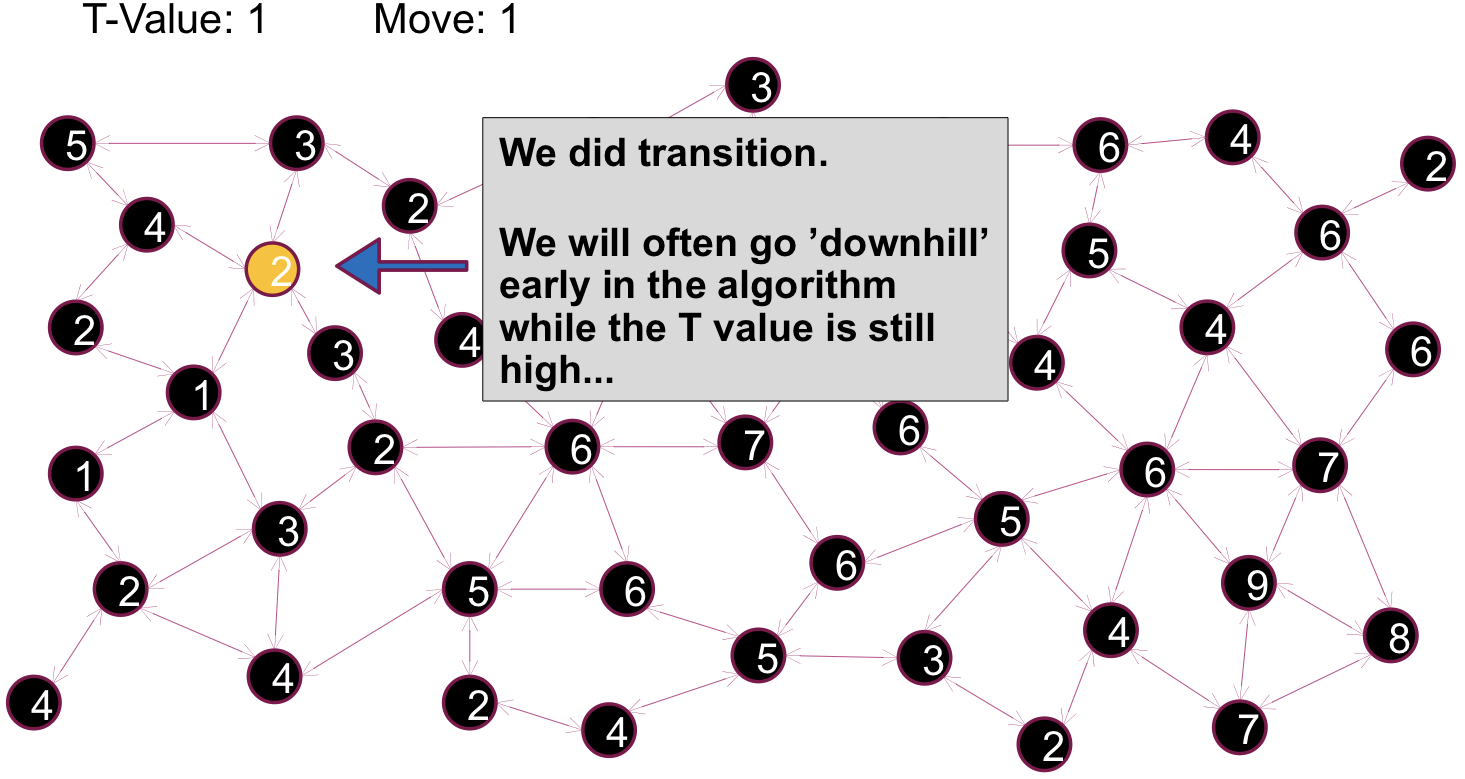
• At each step, out transition function randomly selects a single neighbor node to potentially transition to

  💡

  initial state를 random하게 고른다는 점에서 Greedy Hill Climb with Random Restart과 유사점을 찾을 수 있다.

• Given our current node, n, and the selected neighbor node, m, the algorithm will decide whether to transition from n to m probabilistically. Typically we make the transition with probability 1 if m is fitter than n. Otherwise, the chance that we make the transition depends on the relative fitness of n and m and on a tuning parameter, called the temperature, or t

  💡

  즉 다시 말해서 현재 상태보다 fitter하면 무조건 옮긴다는 측면에서는 Greedy Hill Climb방식과 유사하지만 현재 상태가 더 좋으면 아얘 이동하지 않는 것이 아니라 probablistic하게 탈출할 가능성을 줌으로써 Greedy Hill Climb의 문제점을 해소해보고자 하는 것이다.

• t gradually approaches 0 according to a specified schedule, and the chances of choosing to a less fit state approaches 0 as t approaches 0

  💡

  즉 초반에는 slope를 내려가는 것을 허용했다가 점차적으로 계속해서 더 좋은 쪽으로만 converge하게끔 보정하는 것이다.

💡

Annealing은 특정 이상 온도에서 오랫동안 금속을 노출시켜서 금속을 더 부드럽게 만드는 작업을 의미하는 전문용어이다. 여기에서는 초반에는 less fitter해도 이동하는 것을 허용하고 후반으로 갈수록 허용하지 않는다는 점에서 이러한 용어를 채택하였다.

💡

이후 과정은 동일한 과정의 반복이다. 눈여겨 보아야할 지점은 시간이 지남에 따라서 downhill을 선택할 가능성이 줄어들기는하지만, 초반에는 local optima에 갇히는 문제를 해결해줄 수 있는 가능성을 제공해준다는 점에서 이전 접근방법과 차이를 보인다.

하지만, 물론 이 방식에도 한계가 존재한다.

이러한 측면때문에 다양한 cooling schedule이나 transition function을 적용하는 algorithm이 등장하게 되었다.

Local Beam Search

• We select n initial nodes. Each of these will be termed a particle

• At each step
  • Create a set, S, of nodes consisting of the nodes the particles are currently at and the neighbors of these nodes
  • The particles transition to the n fittest nodes in S

• The search terminates when no transitions are made

💡

즉, 다시 말해서 지속적으로 n개의 노드들의 이웃까지 포함해서 최적해를 지속적으로 고르는 방식이다.

💡

종료는 converge했을 때 진행해주면 된다.

Certainly do not assume that Local Beam Search is better than Simulated Annealing. They both have advantages and disadvantages

• Disadvantages of Local Beam Search

  → All the particles ended up clustered together

💡

The idea was to use Local beam search to get a greater awareness of the state space than Greedy hill climb provided. This clustering behavior limits the effectiveness of this strategy.

Stochastic Local Beam Search

• We select n initial nodes. Each of these will be termed a particle

• At each step
  • Create a set, S, of nodes consisting of the nodes the particles are currently at and the neighbors of theses nodes
  • The particles transition to n nodes in S drawn at random but weighted by their relative fitness

• The search terminates when no neighbor node is better than any of the current nodes

💡

Avoids the clustering issue of LBS and is generally preferable

💡

즉 Local Beam Search에서는 가장 좋은 n개의 상태를 결정적으로 선택했다면, Stochastic Local Beam Search는 이를 확률적으로 선택함으로서 좋지 않은 해를 갖는 상태가 다음 상태로 진행될 가능성을 열어두게 된다. 이를 통해 cluster되는 issue를 alleviate한 것이다.

Search Scenario 3

Find an optimal path (in terms of the cost function) from a given origin state to a given goal state

• The search space is finite

• The search space and edge costs are known

• The search space is layered

  → The nodes at which an n-step path from the origin terminates are disjoin. The search space and edge costs are known

💡

즉, 다시 말해서 topological sort가 가능하기 때문에 DP를 사용할 수 있게 된다.

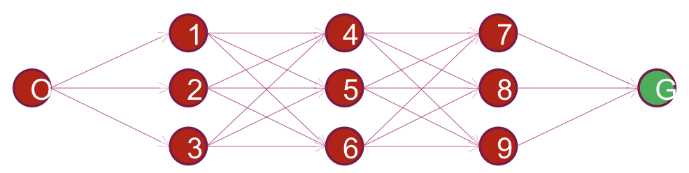
Dynamic Programming for Path Finding

1. Assign the origin the value 0

2. Proceed iteratively through each layer, L, of the state space. Treat the origin as the 0 layer and begin at layer 1:
   1. Where is the value of an edge from node m to node n, assign each node n in L the value
   2. Add a pointer from the node m that minimizes the above equation to n

3. Backtrack from the Goal to the origin using these pointer to find the optimal path

💡

그냥 DP통해서 업데이트 해준다고 생각해주면 된다. 이게 가능한 가장 큰 이유는 topological sort가 된 상태이기 때문에 순서를 강제할 수 있기 떄문이다.