13. Dimensionality Reduction

Curse of Dimensionality

Datasets are typically high-dimensional

→ 차원이 올라갈수록 영역당 observation이 줄게 된다. 또한, computational cost가 올라가게 된다. 이러한 현상을 curse of dimensionality 라고 한다.

Observed Dimensionality

실제로 data가 놓여있는 공간의 dimension은 그보다 더 작다.

Dimensional Reduction

기존 데이터들의 properties들을 보존하면서 high-dimensional space를 low-dimensional space로 내리고자 하는것

→ It is commonly used for

1. feature extraction

2. data compression

3. data visualization

Linear dimensionality reduction

1. Principal component analysis (PCA)

2. Factor analysis

Non-linear dimensionality reduction

1. Kernel principal component analysis (Kernel PCA)

2. T-SNE

Linear Dimensionality Reduction

Data Projection into Subspace

We need to find a new basis of 2D space that can carry most of the information

→ 그렇다면 어떤 기준으로 basis를 정해야하는 것인가?

이에 대한 기준 2가지를 순서대로 살펴보도록 하자.

Criteria 1 : Maximum Variance Formulation

Given a dataset $\{x_n\}_{n = 1}^N$ where $x_n\in \R^D$, the goal is to project the data onto a space having dimensionality $M < D$ while maximizing the variance of the projected data.

첫 번째 기준은 data들의 variance가 가장 크게끔 basis를 설정하는 것이다. 구체적인 상황을 1차원에서 확인하고, 이를 다차원으로 확장시켜보도록 하자.

1-dimensional Principal Subspace

$x_n$을 $u$에 projection 시키고자 하는 것 $u^Tx_n\in \R^1$

The variance of the projected data is given as

$$\frac{1}{N}\sum_{n = 1}^N(u^Tx_n - u^T\bar x)^2 = u^TSu \\ \text{where }S = \frac{1}{N}\sum_{n = 1}^N(x_n-\bar x)(x_n-\bar x)^T$$

이때, S를 Empirical covariance matrix of the data 라고 부른다.

• Proof

  We are asked to prove that

  $$\frac{1}{N}\sum_{n = 1}^N(u^Tx_n - u^T\bar x)^2 = u^TSu$$

  where $x_n$ is the n-th data point in the dataset, $\bar{x}$ is the mean of the data set, $u$ is a vector, and $S$ is the covariance matrix of the data set.

  To start, expand the square in the left-hand side (LHS) of the equation:

  $$\frac{1}{N}\sum_{n = 1}^N(u^Tx_n - u^T\bar x)^2 \\ =\frac{1}{N}\sum_{n = 1}^N(u^Tx_n)^2 - 2(u^Tx_n)(u^T\bar{x}) + (u^T\bar{x})^2 \\ =\frac{1}{N}\sum_{n = 1}^N(u^Tx_n)^2 - 2(u^T\bar{x})\frac{1}{N}\sum_{n = 1}^N(u^Tx_n) + \frac{1}{N}\sum_{n = 1}^N(u^T\bar{x})^2 \\ =\frac{1}{N}\sum_{n = 1}^N(u^Tx_n)^2 - 2(u^T\bar{x})(u^T\bar{x}) + (u^T\bar{x})^2 \\ =\frac{1}{N}\sum_{n = 1}^N(u^Tx_n)^2 - (u^T\bar{x})^2$$

  Now, let's work on the right-hand side (RHS) of the equation:

  $$u^TSu = u^T\left(\frac{1}{N}\sum_{n=1}^{N}(x_n-\bar{x})(x_n-\bar{x})^T\right)u \\ = u^T\left(\frac{1}{N}\sum_{n=1}^{N}x_nx_n^T - \frac{1}{N}\sum_{n=1}^{N}x_n\bar{x}^T - \frac{1}{N}\sum_{n=1}^{N}\bar{x}x_n^T + \frac{1}{N}\sum_{n=1}^{N}\bar{x}\bar{x}^T\right)u \\ = \frac{1}{N}\sum_{n=1}^{N}u^Tx_nx_n^Tu - \frac{1}{N}\sum_{n=1}^{N}u^Tx_n\bar{x}^Tu - \frac{1}{N}\sum_{n=1}^{N}u^T\bar{x}x_n^Tu + \frac{1}{N}\sum_{n=1}^{N}u^T\bar{x}\bar{x}^Tu\\ = \frac{1}{N}\sum_{n=1}^{N}(u^Tx_n)^2 - \frac{1}{N}\sum_{n=1}^{N}(u^Tx_n)(u^T\bar{x}) - \frac{1}{N}\sum_{n=1}^{N}(u^T\bar{x})(u^Tx_n) + \frac{1}{N}\sum_{n=1}^{N}(u^T\bar{x})^2 \\ =\frac{1}{N}\sum_{n=1}^{N}(u^Tx_n)^2 - 2(u^T\bar{x})(u^T\bar{x}) + (u^T\bar{x})^2$$

  As you can see, the LHS and the RHS are the same, which completes the proof.

💡

왼쪽이 quadratic form이므로 그에 대응되는 self-adjoint인 S가 존재한다. $S \in M^{D \times D}$. 또한 $S$는 self-adjoint하므로 Real-digonalizable하다. 또한 covariance matrix이므로 positive semi-definite이다. 즉 S는 non-negative eigenvalue만을 가진다.

PCA can be formulated as

$$\max_{u\in \R^D}u^TSu \text{ subject to }u^Tu = 1$$

Lagrange multiplier를 적용하면

$$L = u^TSu - \lambda(u^Tu - 1) \\ \Rightarrow Su = \lambda u$$

즉 $u$ must be the eigenvector of S having eigenvalue$\lambda$

따라서

$$\max_{u\in \R^D}u^TSu = \lambda$$

💡

Variance를 최대로 하는 PCA는 Empirical covariance matrix의 가장 큰 eigenvalue에 대응되는 eigenvector를 basis로 설정해주면 된다.

M-dimensional Principal Subspace

이를 확장시켜서 basis를 $M$개 잡아보도록 하자.

Let $\{u_1, \dots, u_M\}$ is a basis. PCA can be given as the maximization of total variance

$$\max_{\{u\}_1^M\in \R^{D}}\sum_{m = 1}^M u_m^TSu_m \\\text{subject to }u_i^Tu_j = \delta_{ij}$$

→ 여기서 $S \in M^{D \times D}$

1차원에서와 동일하게 Lagrange multiplier를 처리하게 되면 다음과 같은 결론을 얻을 수 있다.

💡

Variance를 최대로 하는 PCA는 Empirical covariance matrix의 가장 큰 M개의 eigenvalue에 대응되는 eigenvector를 basis로 설정해주면 된다.

Criteria 2 : Minimum Error Formulation

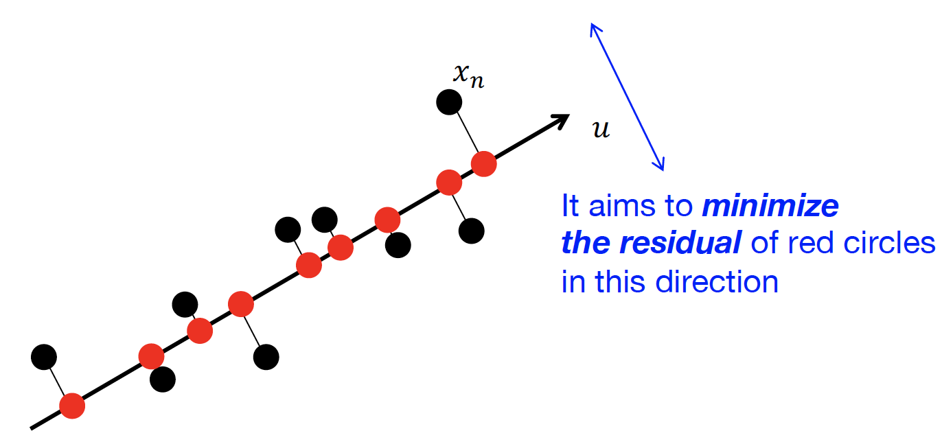
두 번째 기준은 정보의 손실을 최소로 하는 것이다. 즉 다음과 같은 projection error를 최소화하게끔하는 basis를 찾는 것이 목표이다.

→ 즉, projection matrix를 구하고 싶다고 이해해도 무방하다.

💡

결과적으로 m개의 basis를 잡고, m차원의 subspace에 data를 projection시키고 싶다고 생각해주면 된다.

$$J = \frac{1}{N}\sum_{n = 1}^N\|x_n-\tilde x_n\|^2$$

이때 우리는 다음과 같은 orthonormal basis를 잡았다고 가정하자.

(사실 Gram-schimdt를 활용하면 쉽게 orthonormal basis를 잡을 수 있다.)

$$\text{basis : }\{u_1,\dots, u_D)$$

그리고 일반성을 잃지 않고, 우리가 원하는 subspace의 basis를 $\{u_1, \dots, u_M\}$이라고 하자.

선형대수적인 지식을 활용하면 $J$를 작게 만들고 싶다는 의미는 결과적으로는 다음과 같이 정리할 수 있다.

$$J = \frac{1}{N}\sum_{n = 1}^N\sum_{i = M + 1}^D(x_n^Tu_i-\tilde x^Tu_i)^2 = \sum_{i = M + 1}^D u_j^TSu_j$$

그러면 다음과 같은 최적화 문제로 바뀌게 된다.

$$\min_{u\in \R^{D\times M}}\sum_{i = M + 1}^D u_m^TSu_m \\\text{subject to }u_i^Tu_j = \delta_{ij}$$

💡

Error를 최소로 하는 PCA는 Empirical covariance matrix의 가장 작은 D - M개의 eigenvalue에 대응되는 eigenvector를 projection subspace의 basis로 설정해주면 된다.

또한, 일반적으로 projection subspace의 basis를 principal component 라고 부른다.

PCA for High-Dimensional Data

일반적으로 dimension $D$에 비해서 data point의 개수 $N$이 작을 경우 dataset이 high-dimensional라고 부른다.

이때, empirical covariance matrix $S$의 eigenvalue decomposition을 하려면 결과적으로 $O(D^3)$의 시간복잡도가 걸린다. (왜냐하면 $S \in M^{D \times D}$)

하지만, 잘 생각해보면 $D$ 차원에 데이터가 $N$개가 있는 상황이므로, 데이터들이 형성할 수 있는 subspace는 기껏해봐야 $N$차원이다. 즉 dataset이 high-dimensional인 경우, $S$의 eigenvalue가 대부분 0이라는 것을 추측할 수 있다.

이러한 특성을 활용하면 data의 개수에 비해서 차원이 큰 경우에 computational cost를 줄일 수 있다.

$$S = \frac{1}{N}X^TX$$

💡

$X$는 n번째 행이 $x_n - \bar x$ 인 matrix이다.

💡

이때 S를 sample covariance matrix라고 부른다. 정확하게는 각 차원들끼리의 covariance에 대한 정보를 담고 있는 배열이다.

일단 $S$를 다음과 같이 표현할 수 있고, 이를 활용하면 $S$의 eigenvalue를 구하는 과정을 다음과 같이 표현할 수 있다.

$$\frac{1}{N}X^TXu_i = \lambda_iu_i$$

양변에 $X$를 곱해주면 다음과 같다.

$$\frac{1}{N}XX^TXu_i = \lambda_iXu_i$$

즉 $XX^T$의 eigenvector와 eigenvalue를 구하는 문제로 바뀌었다. 이때, 편의를 위해 $Xu_i = v_i$라고 치환하자

$$\frac{1}{N}XX^Tv_i = \lambda_iv_i$$

$XX^T$의 eigenvalue와 eigenvector를 구함으로써 $v_i$를 구했다고 하자. 그렇다면 이거를 활용해서 $u_i$로 어떻게 복원할 것인가?

위 식에 다시 $X^T$를 곱해보자

$$\frac{1}{N}X^TXX^Tv_i = \lambda_iX^Tv_i \\ = \frac{1}{N}X^TXX^TXu_i = \lambda_iX^Tv_i$$

이때, $\frac{1}{N}X^TXu_i = \lambda_iu_i$이므로

$$\frac{1}{N}X^TXX^TXu_i = \lambda_iX^Tv_i \\ \Rightarrow \lambda_iX^TXu_i = \lambda_iX^Tv_i \\ \Rightarrow N(\lambda_i)^2u_i = \lambda_iX^Tv_i$$

따라서

$$u_i = \frac{1}{N\lambda_i}X^Tv_i$$

즉 이렇게 하면 시간복잡도를 $O(N^3)$로 낮출 수 있다. 왜냐하면 결과적으로 $XX^T \in M^{N \times N}$ 이기 때문이다.

Factor Analysis

Factor analysis(FA) 및 probabilistic PCA (PPCA)는 generative model이다. 반면 앞에서 다룬 PCA는 데이터들이 놓여있는 차원보다 단순히 더 낮은 subspace로 projection시킨 것에 불과하다.

예를 들어 위 예시를 보면, 사람이라면 각 cluster에 대해 projection을 다르게 진행해야한다는 점을 판단할 수 있다. 하지만, PCA는 이러한 판단을 할 수 없다. 반면, factor analysis는 data의 distribution을 찾는 generative model이기 때문에 가능하다.

💡

즉, PCA는 단순히 data compression의 역할만 수행할 수 있다.

Revisit Mixture of Gaussian

Mixture of Gaussian의 경우 data가 놓여있는 차원보다 데이터의 수가 많이 작은 경우에 사용하기가 부적합하다.

예를 들어 $x \sim \mathcal N(\mu, \Sigma)$ 라고 가정하자. (단순히 1개의 Gaussian이라고 생각하자.)

이에 대한 MLE는 다음과 같을 것이다.

$$\mu = \frac{1}{n}\sum_{i = 1}^n x^{(i)} \\ \Sigma = \frac{1}{n}\sum_{i = 1}^n (x^{(i)} - \mu)(x^{(i)}-\mu)^T$$

이때, 데이터들이 놓인 차원보다 데이터들의 개수가 더 적다고 가정하면 covariance matrix인 $\Sigma$ 가 singular가 된다.

$$\frac{1}{(2\pi)^{k/2}|\Sigma|^{-1/2}}\exp\{-\frac{1}{2}(\textbf{x}-\mathbf{\mu})^T\Sigma^{-1}(\textbf{x}-\mathbf{\mu})\}$$

이렇게 되면 Multivariable Gaussian distribution을 계산하기가 어려워진다.

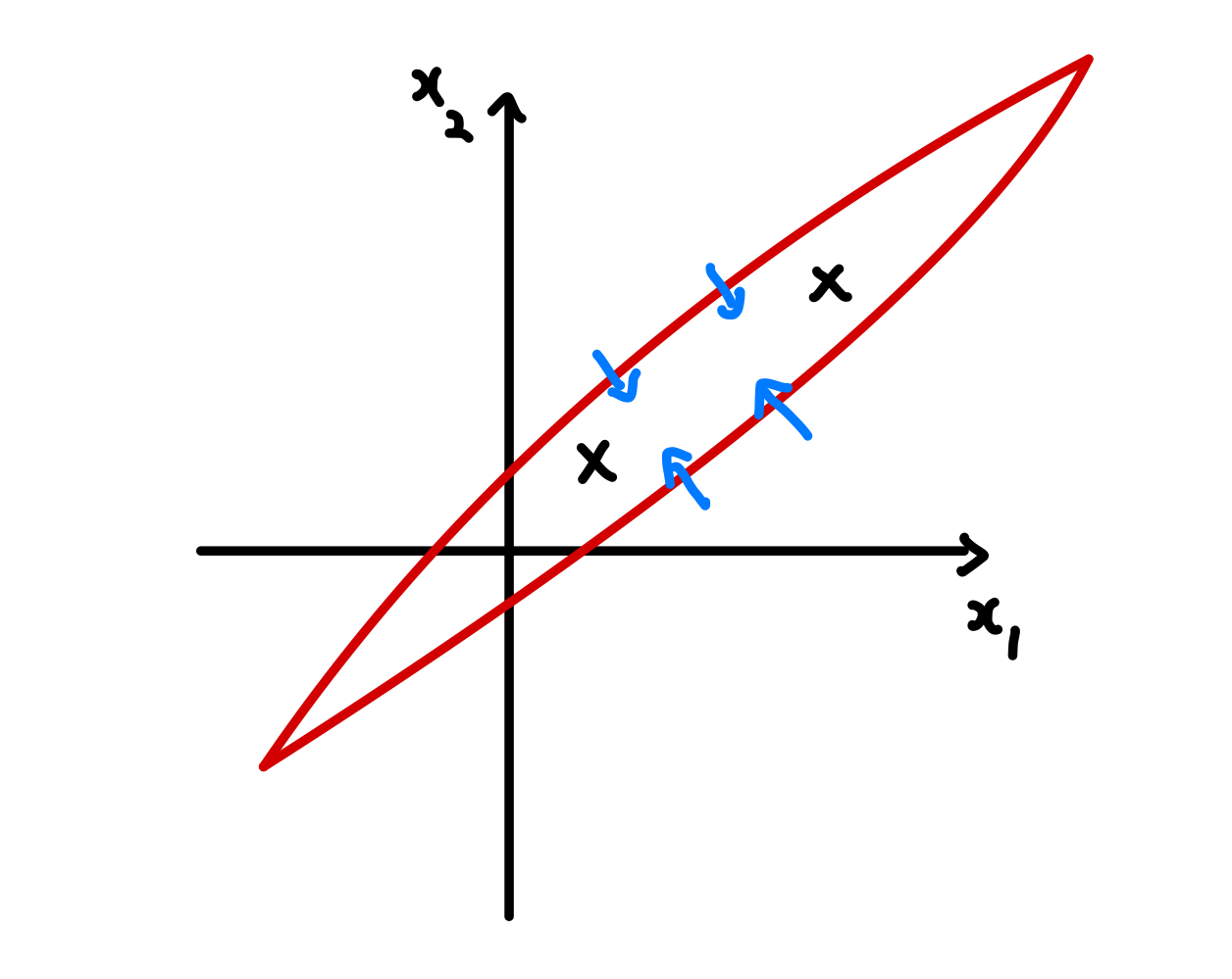
추가적으로 만약 2개의 2차원 상에 존재하는 데이터가 존재하고, Multivari-Gaussian 1개를 통해 데이터들의 분포를 추정하고 싶다고 가정하자. 그러면 Mixture of Gaussian에 의해서 추정되는 Gaussian은 굉장히 flat한 형태의 Gaussian이 될 것이다. 이러한 측면으로 봐도 covariance matrix가 singular가 된다는 것을 확인할 수 있다.

💡

거의 사실상 Gaussian이 직선이 될 것이고, 해당 직선을 살짝만 벗어나도 확률이 0이 될 것이다. 즉 좋은 모델링이 아니다.

만약 여전히 Mixture of gaussian을 쓰고 싶은 경우에는 어떻게 해야할까? 정답은 $\Sigma$에 restriction 을 주면 된다.

Option 1 : $\Sigma$ to be diagonal

위 그림에서 확인할 수 있는 것처럼, covariance가 diagonal로 제한하게 되면 비스듬하게 Gaussian이 형성되지 않게끔 한다. MLE를 통해 covariance를 추정한 결과는 다음과 같다.

$$\Sigma_{jj} = \frac{1}{n}\sum_{i = 1}^n (x_j^{(i)} - \mu_j)^2$$

하지만, 각 feature가 uncorelated되어 있다는 가정을 하게 되는 꼴이므로 문제가 발생할 수 있다.

Option 2 : $\Sigma = \sigma^2I$

Option 2는 Option 1에 비해서 더 강한 가정을 하고 있다.

이렇게 되면 Gaussian는 Circular 형태를 띄게 된다. MLE를 통해 $\sigma^2$를 esimate한 결과는 다음과 같다.

$$\sigma^2 = \frac{1}{nd}\sum_{j = 1}^d\sum_{i = 1}^n(x_j^{(i)} - \mu_j)^2$$

💡

사실 covariance의 diagonal들을 평균 취해준 것에 불과하다.

앞서 살펴본 것처럼, option 1 과 option 2는 feature들 사이의 관계를 무시하게 되는 문제점이 존재하게 된다. 이를 해결하기 위해서 등장한 개념이 factor analysis이다.

Definition of Factor analysis

Factor analysis is a statistical method used to describe variability among observed, correlated variables in terms of a potentially lower number of unobserved variables called factors. For example, it is possible that variations in six observed variables mainly reflect the variations in two unobserved (underlying) variables. The observed variables are modeled as linear combinations of the potential factors plus error terms

즉, 결과적으로 latent variable들의 linear combination과 error term들의 합으로 observed data를 표현하고 싶은 것이다.

💡

이러한 측면에서 factor들의 개수($z$의 dimension)은 실질적으로 $x$가 놓여있는 subspace의 dimension과 관련이 되어있다. 추가적으로 noise를 줌으로써 살짝의 smoothing을 취하고자 하는 것.

Exact procedure

일단 다음과 같이 가정한다.

$$z\sim \mathcal N(0, I) \text{ where } z\in \R^k \\ x = \mu + \Lambda z + \epsilon \text{ where } x\in \R^d\\ \epsilon \sim \mathcal N(0, \Psi) \text{ where } \epsilon\in \R^n$$

💡

parameters : $\mu \in \R^d, \Lambda \in \R^{d \times k}, \Psi \in R^{d \times d}$ (where $\Psi$ is Diagonal)

💡

$k$는 data가 살고 있을 것으로 추정되는 차원과 관련이 되어있다. 즉 $x$는 $\R^d$에 살고 있지만 실질적으로는 dimension이 $k$인 subspace상에 놓여있다고 생각하는 것. 결과적으로 k는 데이터가 놓여있을 것이라고 생각하는 차원만큼 설정하는 hyper-paramter이다.

따라서

$$x|z \sim \mathcal N(\mu+\Lambda z, \Psi)$$

💡

$z$가 주어지면 사실상 $\mu + \Lambda z$ 는 constant이고, $\epsilon$에 의해서 perturbation되는 것으로 이해할 수 있다.

💡

$z\in \R^k$이므로 사실상 latent variable이 k개라고 생각해주면 된다. Mixture of gaussian의 경우는 latent variable이 1개이고, latent variable의 class가 k개라고 가정했다는 것을 주의하도록 하자.

💡

추가적으로 $\Psi$를 diagonal로 잡았기 때문에, data의 feature에 대한 noise가 독립이라고 가정한 것이다.

Example 1

$z \in \R^1, x\in \R^2(k = 1, d = 2, n = 7)$

💡

$k$는 latent variable의 차원(실제 data가 살고 있는 차원이랑 관계가 있음), $d$은 data의 차원, $n$은 data의 개수

이때

$$\Lambda = [2, 1]^T \\ \mu = [0,0]^T$$

라고 하자. 위 상황을 기하학적으로 나타내면 다음과 같다.

💡

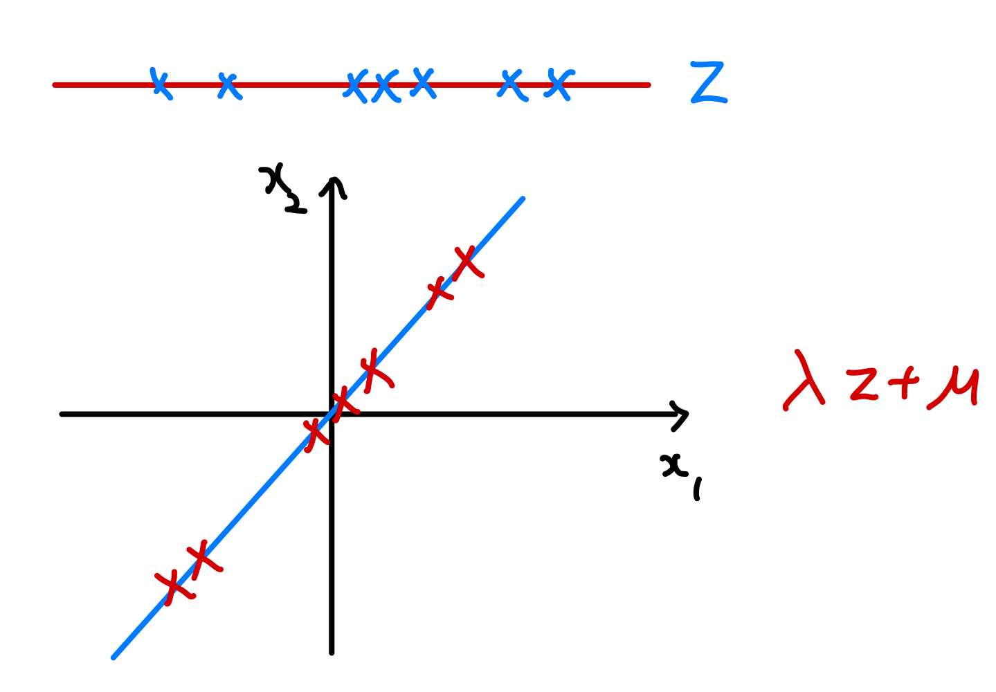
각 data에 대응되는 latent variable의 값이 존재한다고 이해해야 한다. 위 상황에서는 data가 총 7개라고 가정했으므로, z의 값도 7개인 것이다.

추가적으로 $\Psi$가 다음과 같다고 하자.

$$\Psi = \left[ {\begin{array}{cc} 1 & 0 \\ 0 & 2 \\ \end{array} } \right]$$

그러면 error에 대한 distribution은 다음과 같을 것이다.

(이때 가로는 $x_1$, 세로는 $x_2$를 의미하게 된다.)

error까지 더해준 결과는 다음과 같다.

이때 분홍색으로 표기한 점이 위의 model로부터 생성된 sample이다.

💡

즉, 실제의 data를 기반으로 $\mu, \Lambda, \Psi$를 optimize하고 이를 통해 data의 distribution을 예측한다고 이해하면 된다. 즉, $z$를 sampling함으로써 $x$를 sampling하는 효과를 가져올 수 있게 된다. (사실상 data의 distribution을 추정하고 있는 작업이다.)

위 상황에서는 data는 2차원 공간안에 살고 있음에도 불구하고, 실질적으로는 굉장히 적은 차원에서 살고 있다. 따라서 그보다 작은 공간으로 projection시키되, 일종의 noise를 살짝 줌으로써 smoothing한 것으로 이해하면 된다.

Example 2

$z \in \R^2, x\in \R^3(k = 2, d = 3, n = 5)$

💡

$k$는 latent variable의 차원 (실제 data가 살고 있는 차원이랑 관계가 있음), $d$은 data의 차원, $n$은 data의 개수

이를 $\Lambda$와 $\mu$를 활용해서 linear transformation해준 결과를 기하학적으로 나타내면 다음과 같다.

💡

즉 고차원으로 올려준 효과라고 생각해주면 된다.

마지막으로 여기에 noise를 더해주면 다음과 같다.

앞서 2개의 예시에서 살펴본 것처럼, factor-analysis를 사용하면 high-dimensional data를 활용할 수 있게 된다.

Marginals and Conditional of Gaussian Distribution

Suppose $x \sim \mathcal N(\mu, \Sigma)$ where

$$x = \begin{bmatrix} x_1 \\ x_2 \end{bmatrix}$$

where $x_1\in \R^r, x_2\in \R^s, x = \R^{r + s}$ and

$$\mu = \begin{bmatrix} \mu_1 \\ \mu_2 \end{bmatrix} , \Sigma = \begin{bmatrix} \Sigma_{11} & \Sigma_{12} \\ \Sigma_{21} & \Sigma_{22} \end{bmatrix}$$

💡

이때 $\Sigma$는 covariance matrix이므로 symmetric하다. 따라서 $\Sigma_{12} = \Sigma_{21}$

First, we want to compute the marginal distribution of $x_1$(i.e $p(x_1)$).

By the definition

$$p(x_1) = \int p(x_1, x_2)dx_2 \\ = \int \frac{1}{(2\pi)^{n/2}|\Sigma|^{1/2}}\exp(-\frac{1}{2}\begin{pmatrix} x_1 -\mu_1 \\ x_2 - \mu_2 \end{pmatrix}^T \begin{pmatrix} \Sigma_{11} & \Sigma_{12} \\ \Sigma_{21} & \Sigma_{22} \end{pmatrix}^{-1} \begin{pmatrix} x_1 -\mu_1 \\ x_2 - \mu_2 \end{pmatrix})dx_2$$

So we can easily show that

$$x_1 \sim\mathcal N(\mu_1, \Sigma_{11})$$

Secondly, we want to compute the conditional distribution of $x_1|x_2$

By the definition

$$p(x_1|x_2) = \frac{p(x_1, x_2)}{p(x_2)}$$

So we can easily show that

$$x_1|x_2 \sim \mathcal N(\mu_{1|2}, \Sigma_{1|2}) \text{ where} \\ \mu_{1|2} = \mu_1 + \Sigma_{12}\Sigma_{22}^{-1}(x_2 - \mu_2) \\ \Sigma_{1|2} = \Sigma_{11} - \Sigma_{12}\Sigma_{22}^{-1}\Sigma_{21}$$

💡

특히 conditional distribution 공식은 외우지 말고, 필요할때마다 참고하는 식이면 충분하다.

정확한 증명은 다음 사이트를 참고하면 된다.

Conditional distributions of the multivariate normal distribution

The Book of Statistical Proofs – a centralized, open and collaboratively edited archive of statistical theorems for the computational sciences

https://statproofbook.github.io/P/mvn-cond.html

EM Algorithm for Factor Analysis

1. Derive $p(x, z)$

$$\begin{bmatrix} z \\ x \end{bmatrix} \sim \mathcal N(\mu_{x,z}, \Sigma) \\ z \sim \mathcal N(0, I) \\ x = \mu + \Lambda z + \epsilon$$

💡

$p(x, z)$가 gaussian이라고 가정한 것이다.

Since

$$\mathbb E(x) = \mathbb E(\mu + \Lambda z + \epsilon) = \mathbb E(\mu) = \mu \\ \mathbb E(z) = 0$$

$$\mu_{x, z} = \begin{bmatrix} \mu \\ 0 \end{bmatrix}$$

where $\mu \in \R^d, 0 \in \R^k$

Similarly, we can derive

$$\Sigma = \begin{bmatrix} \Sigma_{11} & \Sigma_{12} \\ \Sigma_{21} & \Sigma_{22} \end{bmatrix} \\= \begin{bmatrix} \mathbb E[(z - \mu_z)(z - \mu_z)^T] & \mathbb E[(z - \mu_z)(x - \mu_x)^T] \\ \mathbb E[(x - \mu_z)(x - \mu_z)^T] & \mathbb E[(x - \mu_x)(x - \mu_x)^T] \end{bmatrix}$$

💡

여기서 $\Sigma$는 Sample covariance matrix이다.

Let's calculate one of the elements $\Sigma_{22}$ in the above covariance matrix.

$$\Sigma_{22} = \mathbb E[(x-\mu_x)(x - \mu_x)^T] \\ = \mathbb E[(\Lambda z + \mu + \epsilon - \mu)(\Lambda z + \mu + \epsilon - \mu)^T] \\ = \mathbb E[(\Lambda z + \epsilon)(\Lambda z+ \epsilon )^T] \\ = \mathbb E[\Lambda zz^T\Lambda^T + \Lambda z\epsilon^T + \epsilon z^T\Lambda^T+ \epsilon\epsilon^T]$$

Since, $z$ and $\epsilon$ are not correlated and their expectations are 0,

$$E[\Lambda zz^T\Lambda^T + \Lambda z\epsilon^T + \epsilon z^T\Lambda^T+ \epsilon\epsilon^T] \\ = E[\Lambda zz^T\Lambda^T] +\mathbb E[ \epsilon\epsilon^T] \\ = \Lambda E[zz^T]\Lambda^T + \mathbb E[\epsilon\epsilon^T] \text{ (by linearity)} \\ = \Lambda I\Lambda^T + \Psi \\ = \Lambda\Lambda^T+\Psi$$

By doing similar calculations, we can easily find that

$$\Sigma = \begin{bmatrix} I & \Lambda^T \\ \Lambda & \Lambda\Lambda^T + \Psi \end{bmatrix}$$

Finally, we can derive

$$\begin{bmatrix} z \\ x \end{bmatrix} \sim \mathcal N(\begin{bmatrix} \mu \\ 0 \end{bmatrix},\begin{bmatrix} I & \Lambda^T \\ \Lambda & \Lambda\Lambda^T + \Psi \end{bmatrix})$$

💡

이 식을 통해 likelihood $p(x;\mu, \Lambda, \Psi)$를 구하는 것은 가능하다. 하지만, log-likelihood을 maximize하는 closed-form solution이 존재하지 않는다. 따라서 EM algorithm을 통해 iterative하게 구하고자 하는 것이다.

2. E-step

$$Q_i(z^{(i)}) = p(z^{(i)}|x^{(i)};\Theta)$$

💡

mixture of Gaussian에서는 $z$가 discrete였지만, 여기서는 continuous random variable이다.

💡

EM algorithm에서 살펴본 것처럼, $Q_i(z^{(i)})$를 $p(z^{(i)}|x^{(i)};\theta)$로 잡음으로써 log-likelihood의 lower-bound를 tight하게 만들 수 있다.

Mixture of Gaussian의 경우에는 $p(z^{(i)}|x^{(i)};\Theta)$를 적당히 summation해서 구할 수 있었다. 하지만 여기서는 $z$가 continuous random variable이기 때문에, 위에서 증명한 conditional distribution of gaussian 공식을 활용해야 한다.

$$z^{(i)}|x^{(i)} \sim \mathcal N(\mu_{z^{(i)}|x^{(i)}},\Sigma_{z^{(i)}|x^{(i)}}) \\ \Rightarrow \mu_{z^{(i)}|z^{(i)}} = \Lambda^T(\Lambda\Lambda^T+\Psi)^{-1}(x^{(i)} - \mu) \\ \Sigma_{z^{(i)}|x{(i)}} = I - \Lambda^T(\Lambda\Lambda^T-\Psi)^{-1}\Lambda$$

위 내용을 활용해서 $Q_i(z^{(i)})$를 표현한다.

$$Q_i(z^{i)}) = \mathcal N(\mu_{z^{(i)}|z^{(i)}}, \Sigma_{z^{(i)}|x{(i)}})$$

3. M-step

M-step에서는 $Q_i(z^{(i)})$를 고정하고 다음 식을 maximize하고 싶은 상황이다.

$$\sum_{i = 1}^n\int_{z^{i}}Q_i(z^{(i)})log\frac{p(x^{(i)}, z^{(i)};\mu, \Lambda, \Psi)}{Q_i(z^{(i)})}dz^{(i)}$$

여기서 하나의 트릭은 적분을 expectation 으로 돌릴 수 있다는 것이다. 즉 위의 식을 다음과 같이 바꿀 수 있다.

$$\sum_{i = 1}^n\mathbb E_{z^{(i)}\sim Q_i}[\log p(x^{(i)}|z^{(i)};\mu, \Lambda, \Psi) + \log(z^{(i)}) -\log Q_i(z^{(i)})]$$

💡

나머지 항들은 $\mu, \Lambda, \Psi$ 에 영향을 받지 않으므로 생략한 것이다.

그러면 결과적으로 각 parameter에 대해서 영향을 주는 것은 $\sum_{i = 1}^n\mathbb E_{z^{(i)}\sim Q_i}[\log p(x^{(i)}|z^{(i)};\mu, \Lambda, \Psi)]$ 가 유일하다.

이때

$$\sum_{i = 1}^n\mathbb E_{z^{(i)}\sim Q_i}[\log p(x^{(i)}|z^{(i)};\mu, \Lambda, \Psi)] \\ = \sum_{i = 1}^n \mathbb E[\log\frac{1}{(2\pi)^{d/2}|\Psi|}\exp(-\frac{1}{2}(x^{(i)}-\mu-\Lambda z^{(i)})^T\Psi^{-1}(x^{(i)}-\mu-\Lambda z^{(i)}))] \\ = \sum_{i = 1}^n \mathbb E[-\frac{1}{2}\log|\Psi| - \frac{n}{2}\log(2\pi)-\frac{1}{2}(x^{(i)}-\mu-\Lambda z^{(i)})^T\Psi^{-1}(x^{(i)}-\mu-\Lambda z^{(i)})]$$

위 식을 각각 $\mu, \Lambda, \Psi$에 대해서 미분하고 0이 나오는 값을 찾아주면 된다. (Quadratic function임을 보장할 수 있으므로 미분하고 0인 값만 찾아줘도 된다.)상당히 복잡한 과정이 있지만 결과만 살펴보자면 다음과 같다.

$$\Lambda = (\sum_{i = 1}^n(x^{(i)}- \mu)\mu_{z^{(i)}|x^{(i)}}^T)(\sum_{i = 1}^n\mu_{z^{(i)}|x^{(i)}}u_{z^{(i)}|x^{(i)}}^T+\Sigma_{z^{(i)}|x^{(i)}})^{-1} \\ \mu = \frac{1}{n}\sum_{i = 1}^nx^{(i)} \\ \Phi = \frac{1}{n}\sum_{i = 1}^nx^{(i)}x^{(i)^T}-x^{(i)}\mu_{z^{(i)}|x^{(i)}}^T\Lambda^T - \Lambda\mu_{z^{(i)}|x^{(i)}}x^{(i)^T}+\Lambda(\mu_{z^{(i)}|x^{(i)}}\mu_{z^{(i)}|x^{(i)}}^T+\Sigma_{z^{(i)}|x^{(i)}})\Lambda^T$$

이때

$$\Psi_{ii} = \Phi_{ii}$$

로 설정한다. 즉 $\Psi$가 Diagonal이 되게끔 하는 것이다.

💡

이때, $\mu$는 parameter가 바뀜에 따라서 변하지 않으므로 한번만 계산해줘도 무방하다.

정확한 유도는 다음을 참고하도록 하자.

cs229-notes9.pdf

Mixture of Factor Analysis

The assumption is that there are a number of different subpopulations (clusters), each of which is modeled with its own factor analysis model. This model is powerful because it can capture complex structures in the data. The factor analysis part allows it to capture correlations in the data, while the mixture model part allows it to represent multiple different subpopulations. This makes it particularly useful for things like clustering high-dimensional data, dimensionality reduction, and exploratory data analysis.

💡

Mixture of Factor Analysis는 linear combination of different factor analysis model로 생각할 수 있다.

먼저 Factor analysis를 다시 확인해보도록 하자.

$$x|z \sim \mathcal N(\mu+\Lambda z, \Psi) \\ p(x) = \int_zp(x|z)p(z) dz$$

즉 결과적으로 $x = \mu + \Lambda z + \epsilon$ 의 형태로 표현이 된다는 것을 가정한 것이다.

반면, Mixture of Factor Analysis는 이와 달리 Factor Analysis들의 linear combination으로 $p(x)$가 표현된다고 가정한다

$$p(x) = \sum_{i = 1}^k \pi_i\int p(x|z_i,\mu_i, \Lambda_i, \Psi_i)p(z_i)dz_i$$

where

$$z_i \sim \mathcal N(0, I) \\ x|z_i \sim \mathcal N(\mu_i+\Lambda z_i, \Psi_i)$$

💡

Mixture of Factor Analysis는 clustering(Mixture model) 과 dimensionality reduction(Factor analysis)를 동시에 수행하게 된다.

Nonlinear Dimensionality Reduction

만약 데이터가 다음과 같이 manifold상에 존재한다면, 단순한 linear pca만으로는 데이터들의 특성을 반영해주기 어렵다. 이러한 문제를 해결하고자 등장한 개념이 non-linear PCA이다.

하나의 더 예시를 살펴보도록 하자.

A better dimensionality reduction can be done by PCA after mapping of data points to feature space.

💡

The feature space is an alternative representation of the original data that is obtained through some transformation or feature extraction process. It aims to capture the relevant information or patterns in a more suitable and informative way for analysis or modeling.

즉 원래 공간에서 차원 축소가 잘 진행되지 않는 형태의 data distribution을 feature space로 transformation시키면 상대적으로 좋은 형태의 차원 축소를 진행시킬 수도 있다는 것

💡

즉 이전의 방법과 거의 동일하나 original data space에서 PCA를 진행하는 것이 아니라, feature space 상에서 PCA를 진행하려고 하는 것이다.

The objective for Kernel PCA

앞서 SVM with kernel에서 살펴본 것처럼, 계산적으로 cost가 크기 때문에 직접적으로 feature space에서 계산하는 것보다는 kernel function를 통해 계산하고자 하는 것이다.

$$K = k(\bold x, \bold y) = \langle \Phi(\bold x), \Phi(\bold y)\rangle = \Phi(\bold x)\Phi(\bold y)^T$$

앞서 PCA에서 했던 작업과 같이 feature space 상에서의 empirical covariance matrix를 구하면 다음과 같다.

💡

결국 covariance matrix의 제일 큰 eigenvalue를 찾는 것이 중요한 문제가 된다.

$$S = \frac{1}{N}\sum_{i = 1}^N(\phi(x_i)-\mu_i)(\phi(x_i) - \mu_i)^T$$

where $M$ : the dimension of feature space

논의의 편의를 위해 평균이 0이라고 가정을 하자. 그러면

💡

정확하게는 평균이 0이 되게끔 조정을 하는 것이다. 일반적인 케이스에 대해서는 뒤에 다루도록 하자.

$$S = \frac{1}{N}\sum_{i = 1}^N\phi(x_i)\phi(x_i)^T$$

그러면 m-dimensional principal subspace를 구성하고자 하는 경우에는 objective가 다음과 같다.

$$\max\sum_{k = 1}^m\lambda_i \text{ (}\lambda_i\text{ is a eigenvalue of }S)$$

즉 $S$의 eigenvalue 중에 가장 큰 m개를 찾는 것이 목표이다.

💡

원하는 크기의 principal subspace의 차원에 의해서, 더해지는 eigenvalue의 개수가 달라지게 된다.

이를 위해서는 일단 $S$의 eigenvector와 eigenvalue를 찾아야 한다. 그런데 식을 잘 관찰해보면 다음과 같은 특성을 확인할 수 있다.

$$\frac{1}{N}\sum_{i = 1}^N\phi(x_i)\phi(x_i)^Tv \\= \frac{1}{N}\sum_{i = 1}^N\langle\phi(x_i), v\rangle\phi(x_i) = \lambda v$$

where $v$ is a eigenvector of $S$.

즉 다시 말해서 $v$는 $\{\phi(x_i)\}_{i = 1}^n$들의 linear combination으로 표현할 수 있다는 의미이다.

💡

즉 $S$의 eigenvector들은 $\{\phi(x_i)\}_{i = 1}^n$들의 linear combination으로 표현할 수 있다

So, there exist some coefficients $\{\alpha_n\}_{n = 1}^N$ such that

$$v = \sum_{i = 1}^N\alpha_i\phi(x_i)$$

By using the above equation,

$$\frac{1}{N}(\sum_{i = 1}^N\phi(x_i)\phi(x_i)^T)(\sum_{j = 1}^N\alpha_j\phi(x_j)) = \lambda(\sum_{i = 1}^N\alpha_i\phi(x_i))$$

양변에 $\phi(x_l)^T$를 곱한다

$$\frac{1}{N}\sum_{i = 1}^N\langle\phi(x_l), \phi(x_i)\rangle\sum_{j = 1}^N\alpha_j\langle\phi(x_i), \phi(x_j)\rangle = \lambda\sum_{i = 1}^N\alpha_j\langle\phi(x_l, \phi(x_i)\rangle \\ \Rightarrow \frac{1}{N}\sum_{i = 1}^NK(l, i)\sum_{j = 1}^N\alpha_jK(i, j) = \lambda\sum_{i = 1}^N\alpha_iK(l, i) \\ \Rightarrow \frac{1}{N}\sum_{i = 1}^N\sum_{j = 1}^N\alpha_jK(l, i)K(i, j) = \lambda\sum_{i = 1}^N\alpha_iK(l, i) \\ \Rightarrow \frac{1}{N}\text{row}_l(K^2\alpha) = \lambda \text{row}_l(K\alpha) \\ \Rightarrow \text{row}_l(K^2\alpha) = \text{row}_l(\lambda NK\alpha) \\ \Rightarrow K^2\alpha = \lambda NK\alpha \text{ (since l is arbitary)}$$

where $\alpha = [\alpha_1 , \dots, \alpha_N]^T$ and $K^2 = KK$ (Matrix multiplication)

여태까지의 흐름을 요약하면 다음과 같다.

$$S = \frac{1}{N}\sum_{i = 1}^N\phi(x_i)\phi(x_i)^T$$

라고 했을 때

$$\max\sum_{k = 1}^m\lambda_i \text{ (}\lambda_i\text{ is a eigenvalue of }S)$$

를 만족하게끔 하는 $\lambda_i$들을 찾고 싶은 것이다. 즉 $S$의 eigenvalue들 중 가장 큰 상위 m개를 택해주면되므로, 우리는 S의 eigenvector와 eigenvalue를 찾는 문제로 바뀌게 된다.

앞에서 증명한 것처럼 해당 문제는 결과적으로는 다음 식을 만족하는 $\alpha$와 $\lambda$를 찾는 문제를 푸는 것과 동치가 된다.

$$K^2\alpha = \lambda NK\alpha$$

💡

즉 feature space에서의 basis들의 coordinate로 변환한 것이다. $v$는 feature space의 원소로 굉장히 untractable한 반면, $\alpha$는 coefficient이므로 계산할만하다._

이제 우리는 위 식을 더 정리하려고 한다.

일단, $K$가 symmetric positive semi-definiteness이다. 즉, 모든 eigenvalue가 non-negative이다. 따라서 $K$는 항상 eigen-decomposable하다. 이때, $K$의 eigenvector를 $\{w_i\}_{i = 1}^N$ 이라고 하고, 이에 대응되는 eigenvalue를 $\{\delta_i\}_{i = 1}^N$이라고 하자. 이때, $\{w_i\}_{i = 1}^N$는 basis를 이루므로

$$\alpha = \zeta_1w_1 + \dots, \zeta_Nw_N$$

를 만족하는 $\{\zeta_i\}_{i = 1}^N$이 존재한다. 따라서

$$K\alpha = K(\zeta_1w_1 + \dots, \zeta_Nw_N) = \delta_1\zeta_1w_1 + \dots + \delta_N\zeta_Nw_N \\ \Rightarrow K^2\alpha = \delta_1^2\zeta w_1 + \dots + \delta_N^2\zeta_Nw_N$$

따라서

$$K^2\alpha = \lambda NK\alpha \Leftrightarrow (\lambda N \delta_1\zeta_1-\delta_1^2\zeta_1)w_1 + \dots + (\lambda N \delta_N\zeta_N - \delta_N^2\zeta_N)w_N = 0$$

Since $w_1, \dots, w_N$ are independent

$$\lambda N\delta_i\zeta_i - \delta_i^2\zeta_i = 0 \text{ for all }i \in [1, N]$$

If $\delta_i \ne 0$,

$$\lambda N\zeta_i = \delta_i\zeta_i \\ \Rightarrow \lambda N\zeta_i w_i = \delta_i\zeta_iw_i \\ \Rightarrow \lambda N\zeta_iw_i = \zeta_iKw_i \\ \Rightarrow K(\zeta_iw_i) = \lambda N(\zeta_iw_i) \text{ for all }i \in [1, N] \text{ if }\delta_i \ne 0 \\ \Rightarrow K\alpha = \lambda N\alpha \text{ if } \delta_i = 0 \text{ then }\zeta_i = 0, \forall i\in[1, N]$$

이때 principal subspace를 구할 때 일반적으로 eigenvalue가 0인 값들에 대해서는 고려하지 않으므로 다음과 같은 식을 푸는 문제로 치환해서 풀 수 있게 된다.

$$K\alpha = \lambda N\alpha$$

이때 $K\in \mathcal L(N, N)$이고 $S\in \mathcal L(M, M)$이다. ($M$은 feature space의 dimension으로 $N < M)$

따라서 feature space 상에서 바로 eigenvalue decomposition을 수행하는 것보다 훨씬 computational적으로 훨씬 유리하다.

💡

즉, kernel matrix를 활용해서 높은 차원의 eigenvalue decomposition을 상대적으로 낮은 차원의 eigenvalue decomposition 문제로 회귀해서 풀 수 있게 된다.

Normalization in Kernel PCA

사실 정확하게 하려면 $v$를 unit-vector로 잡아야 한다. 왜냐하면

$$\max_{u\in \R^D}u^TSu \text{ subject to }u^Tu = 1$$

라고 했을 때

$$\max \lambda \\\text{ where }\lambda \text{ is a eigenvalue of }S$$

결과적으로 우리가 원하는 값이 $\lambda$와 같아지기 때문이다. 따라서 앞의 연산에 추가적으로 $v$가 unit vector라는 constraint를 주어야 한다. 이에 따라 $\alpha$에도 제한이 가해지게 된다.

$$1 = v^Tv = \sum_{i = 1}^N\sum_{j = 1}^N\alpha_i\alpha_j\phi(x_i)^T\phi(x_j) \\ = \sum_{i = 1}^N\sum_{j = 1}^N\alpha_iK(i, j)\alpha_j \\ = \alpha^TK\alpha \\ = \alpha^T\lambda N\alpha$$

Therefore,

$$\|\alpha\|^2 = \frac{1}{\lambda N}$$

즉 다음과 같은 $\lambda$를 찾는 작업으로 바뀌게 된다.

$$K\alpha = \lambda N\alpha \\ \text{subject to }\|\alpha\|^2 = \frac{1}{\lambda N}$$

Compute Nonlinear Components

여태까지의 내용을 총 정리해보도록 하자. 또한 일반성을 잃지 않기 위해 principal subspace의 차원을 m으로 가정하겠다.

💡

$M$ : feature space의 차원, $D$ : data space의 차원, $N$ : data의 개수

Suppose we have a dataset $\{x_i\}_{i = 1}^N$ and this dataset is not easily linearly separable.

We want to increase the dimension by using feature mapping so that this dataset could be easily separable in the feature space. So, our objective is as follows

$$\max_{v_i\in\R^M}\sum_{i = 1}^mv_i^TSv_i \\ \text{subject to }\|v_i\| = 1, \forall i \in [1, m]$$

where

$$S := \frac{1}{N}\sum_{i = 1}^N\phi(x_i)\phi(x_i)^T$$

💡

For mathematical simplicity, we suppose that the sample mean is zero

Since we have some constraints for $v_i$, we have to apply for Lagrange multipliers.

$$\mathcal L(v_1, \dots, v_m) = \sum_{i = 1}^mv_i^TSv_i +\sum_{j = 1}^m\lambda_j(1-v_i^Tv_i)$$

Differentiate it w.r.t $v_i$

$$\nabla_{v_i}\mathcal L(v_1, \dots, v_m) = \nabla_{v_i}(v_i^TSv_i) + \nabla_{v_i}(\lambda_i(1-v_i^Tv_i)) \\ \Rightarrow 2Sv_i -2\lambda_iv_i = 0 \\ \Rightarrow Sv_i = \lambda_iv_i$$

Therefore

$$\max_{v_i\in\R^M}\sum_{i = 1}^mv_i^TSv_i \\ \text{subject to }\|v_i\| = 1, \forall i \in [1, m]$$

is equivalent to

$$\max_{v_i\in\R^M}\lambda_i \\ \text{where } \lambda_i \text{ is eigenvalue of }v_i \\ \text{subject to }\|v_i\| = 1, \forall i \in [1, m]$$

So, this problem is actually the problem of finding the eigenvalue of $S$.

Since $S \in \mathcal L(M, M)$, the computational cost for finding eigenvectors and eigenvalues is very large. We want to reduce the computational cost by using kernel trick

Actually, the problem which we actually want to solve is finding the solution of the following equation

$$Sv_i = \lambda_iv_i \\ \Leftrightarrow \frac{1}{N}\sum_{j = 1}^N\phi(x_j)\phi(x_j)^Tv_i = \lambda_i v_i$$

We can convert this equation as follows

$$\frac{1}{N} \sum_{j = 1}^N\langle\phi(x_j), v_i\rangle\phi(x_j) = \lambda_iv_i$$

This means that $v_i$ can be expressed by the linear combination of $\{\phi(x_i)\}_{i = 1}^N$. We say

$$v_i = \sum_{j = 1}^N \delta_{ij}\phi(x_j)$$

By using this fact, we can convert the problem of $Sv_i = \lambda_iv_i$ to

$$\frac{1}{N}\sum_{j = 1}^N\phi(x_j)\phi(x_j)^T\sum_{k = 1}^N\delta_{ik}\phi(x_k) = \lambda_i(\sum_{j = 1}^N\delta_{ij}\phi(x_j))$$

and multiply $\phi(x_l)^T$ each equation (i.e $l$ is arbitrary)

$$\frac{1}{N}\sum_{j = 1}^N\phi(x_l)^T\phi(x_j)\sum_{k = 1}^N\delta_{ij}\phi(x_j)^T\phi(x_k) = \lambda_i\sum_{j = 1}^N\delta_{ij}\phi(x_l)^T\phi(x_j) \\ \Rightarrow \frac{1}{N}\sum_{i = 1}^N K(l, j)\sum_{k = 1}^N\delta_{ij}K(j, k) = \lambda_i\sum_{j = 1}^N\delta_{ij}K(l, j) \\ \Rightarrow \frac{1}{N}\sum_{j = 1}^NK(l, j)(K\delta_i)_j = \lambda_i\sum_{i = 1}^N\delta_{ij}K(l, j) \\ \Rightarrow \frac{1}{N}K^2\delta_i = \lambda_i\delta_iK \text{ (Since l is arbitrary)} \\ \Rightarrow K^2\delta_i = \lambda_i\delta_i NK$$

where $\delta = [\delta_1, \dots, \delta_N]^T$, $K(i, j) :=$ i, jth component of Kernel matrix

By using some calculations, the above problem could be converted to

$$K\delta_i = \lambda_i N\delta_i$$

In addition, by $\|v_i\| = 1$

$$\|\delta_i\|^2 = \frac{1}{\lambda_i N}$$

Finally, we want to solve this equation

$$K\delta_i = \lambda_i N\delta_i \\ \text{subject to }\|\delta_i\|^2 = \frac{1}{\lambda_i N}$$

Since $\delta_i$ and $v_i$ has 1-1 correspondence, if we know one of them, the other one can be easily calculated. In addition, if we find such $\delta_i$ (i.e. we know the eigenvalue of $\delta_i)$, we can easily calculate the $\lambda_i$ which we actually want to find. As you expected, since $K \in \mathcal L(N, N)$, we can easily find the $\lambda_i$ for $O(N^3)$ not $O(M^3)$.

So our objective is converted as follows

$$\max_{\{\delta_i\}_{i = 1}^m\in \R^N}\sum_{i = 1}^m\frac{w_i}{N} \\ \text{where }w_i \text{ is eigenvalue of }K \text{ w.r.t }\delta_i\\ \text{subject to } \|\delta_i\|^2 = \frac{1}{\lambda_iN}$$

After we find such $w_i$, this means that we actually know $\{v_i\}_{i = 1}^m$. In other words, we find the principal directions in the feature space. So how can we project new data into the subspace that we found?

Let’s say the subspace we found to $E$ and the new data to $x$.

1. We have to convert $x$ to $\phi(x)$ (i.e transform data space to feature space)

2. Project $\phi(x)$ to the subspace we found

$$\text{Proj}_E\phi(x) = \sum_{i = 1}^m\langle v_i, \phi(x)\rangle v_i \\ = \sum_{i = 1}^m\sum_{j = 1}^N \langle\delta_{ij}\phi(x_j), \phi(x)\rangle v_i \\ = \sum_{i = 1}^m(\sum_{j = 1}^N\delta_{ij}K(x_j, x))$$

where $K$ is a Kernel function

💡

Kernel function을 활용하면 고차원 공간에서 내적을 할 필요가 없이 data space상에서 연산을 수행해주면 되므로 computational 측면에서 그렇게 부담이 크지 않다.

Centering in Feature Space

기존의 Kernel matrix는 다음과 같다.

$$K(i, j) := \langle \phi(x_i), \phi(x_j)\rangle$$

이때, feature space에 대응되는 값들의 평균을 0으로 만들고 싶은 상황으로 이해해주면 된다.

$$\tilde\phi(x_n) := \phi(x_n) -\frac{1}{N}\sum_{i = 1}^N\phi(x_i)$$

이를 기반으로 Kernel matrix를 다시 정의해주면 다음과 같다.

$$\tilde K(i, j) := \langle \tilde \phi(x_i), \tilde \phi(x_j)\rangle \\ = \langle\phi(x_i) - \frac{1}{N}\sum_{k = 1}^N\phi(x_k), \phi(x_j) - \frac{1}{N}\sum_{k = 1}^N\phi(x_k) \rangle \\ = K(i, j) -\frac{1}{N}(\sum_{k = 1}^NK(i, k) + K(j, k)) + \frac{1}{N^2} \sum_{i = 1}^N\sum_{j = 1}^NK(i, j)$$

Therefore,

$$\tilde K = K - 1_NK - K1_N +1_nK1_n \\ = (I - 1_N)K(I-1_N)$$

왜냐하면 $1_NK$의 i,j 원소는 j번째 열의 평균, $K1_N$의 i,j 원소는 i번째 행의 평균, $1_NK1_N$은 전체 평균이기 때문이다.

이때, $(I - 1_N) = (I - 1_N)^{-1}$이므로 $\tilde K$는 $K$의 basis change에 대한 결과로 볼 수 있다. 즉 단순히 기저를 변경함으로써 feature space상의 데이터들의 평균을 원점으로 재조정한 것에 불과하다. 또한 $K$는 이미 eigenvalue decomposable하고 기저 변경에 의해서는 eigenvalue를 바꾸지 않으므로 최종적으로 우리의 objective를 다음과 같이 이해할 수 있다.

$$\max_{\{\delta_i\}_{i = 1}^m\in \R^N}\sum_{i = 1}^m\frac{w_i}{N} \\ \text{where }w_i \text{ is eigenvalue of }\tilde K \text{ w.r.t }\delta_i\\ \text{subject to } \|\delta_i\|^2 = \frac{1}{\lambda_iN}$$

💡

여기까지 하면 기존의 평균이 0이라는 가정을 안해도 무방하다.

Isomap

Isomap approximates geodesic distance by using shortest paths in graph

즉 다시 말해서 2개의 data 사이의 metric를 graph 상에서 shortest path로 정의하겠다는 의미이다.

정확하게는 data 사이의 거리가 특정 임계값보다 적으면 edge를 그리고 해당 edge에 가중치를 부여하는 방식으로 그래프를 그린다. 그리고 해당 그래프에서 shortest path 문제를 푸는 것이다.

💡

알고리즘에서 배운 것처럼, shortest path는 metric이 되기 위한 조건을 다 만족한다.

Isomap is a nonlinear dimensionality reduction technique that aims to preserve the global geometric structure of the data. It achieves this by first constructing a neighborhood graph based on pairwise distances between data points and then computing the shortest path distances (geodesic distances) on this graph.

Once the geodesic distances are computed, Isomap creates a new distance matrix that captures the intrinsic relationships between data points in the low-dimensional space. This new distance matrix is constructed by preserving the pairwise distances in the original high-dimensional space, while accounting for the manifold's underlying geometry.

To obtain the low-dimensional representation, Isomap performs eigen-decomposition on the new distance matrix. Eigen-decomposition is a process that decomposes a matrix into its eigenvectors and eigenvalues. In this context, Isomap computes the eigenvectors and eigenvalues of the new distance matrix.

The eigenvectors represent the principal components or basis vectors in the low-dimensional space, and the eigenvalues indicate the importance of each eigenvector in capturing the variance or structure of the data. By selecting a subset of the eigenvectors corresponding to the largest eigenvalues, Isomap obtains the low-dimensional representation of the data.

Autoencoder

앞서 살펴본 것처럼 kernel PCA나 isomap의 경우에는 각 데이터들에 대한 metric을 계산할 필요성이 존재했다. kernel PCA의 경우에는 feature space로 올라감에 따라 계산량이 올라가서 문제였고, isomap의 경우에는 geodesic distance를 구하는 것이 문제가 된다.

→ 따라서 metric을 정의하지 않고 알아서 해줬으면 좋겠다는 측면에서 등장한 개념이 Autoencoder 이다. 즉 data 그 자체로부터 mapping function을 배우게끔 하자는 것이 핵심 아이디어이다.

Encoder는 funciton이며 다음과 같이 정의된다.

$$f : \R^D \to \R^M \\ \text{where }\R^D \text{ is data space, }\R^M \text{ is latent space}$$

즉 다시 말해서 data가 data들의 특성을 반영하고 있는 latent variable $z$에 대응되는 $f$를 찾고 싶은 것이다.

💡

$z$는 $x$에 대한 정보를 최대한 많이 들고 있어야 한다. 즉 $z$만으로 $x$를 다시 만들어낼 수 있어야 한다.

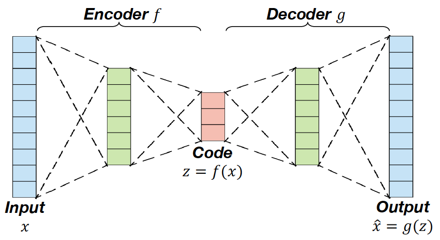
그래서 loss function은 다음과 같이 정의된다.

$$\mathcal L(z) = d(x, g(f(x)) \\ \text{ i.e. }\|x-g(f(x))\|^2$$

이때, encoder $f$와 decoder $g$는 parametric function이 될 수도 있다. 예를 들어 CNN이나 MLP가 그 예시이다.

💡

즉, Neural network를 통해 최적의 Encoder와 Decoder를 찾아낼 수 있다.

예를 들어 이미지의 경우 $f$에 convolution operation을 $g$에 transposed-convolution operation을 취하는 것을 선택할 수 있다.

t-SNE

앞서 살펴본 것처럼, data compression 목적으로 dimensionality reduction을 수행할 때의 가장 큰 목적은 information preserving 이다. 즉 데이터의 정보 손실을 최소화하면서 차원을 축소하고 싶은 것이다.

하지만 t-SNE같은 visualization을 목적으로 dimensionality reduction을 수행할 때의 가장 큰 목적은 similarity preserving 이다.

💡

즉 차원 축소를 하는 목적에 따라 좋은 차원 축소에 대한 기준이 다를 수 있다.

Suppose we have a dataset $\{x_1, \dots, x_N\}$, we want to project a dataset to the lower dimension($\R^2$ or $\R^3$).

이때, t-SNE의 목표는 data space 상에서의 거리($P)$와 projection시킨 space상에서의 거리($Q)$가 최대한 유사하게끔 하고 싶은 것이다. 단 data space상에서의 거리를 정의할 때 gaussian distribution을 사용하고 projection시킨 space상에서 거리는 t-distribution을 사용한 것이다.

💡

이때, t-distribution의 degree of freedom은 1로 설정한다.

이때

$$P_{j|i} = \frac{\exp(-\|x_i-x_j\|^2/2\sigma_i^2)}{\sum_{k \ne i}exp(-\|x_i-x_k\|^2/2\sigma_i^2)} \\ \text{where }p_{i, j} = \frac{p_{j|i}+ p_{i|j}}{2N}(N:\text{\# of data)}$$

💡

$p_{i,j}$를 저런식으로 정의하지 않으면 metric의 조건 중 symmetric이 깨진다. 따라서 이를 보완하기 위해서 평균을 취해주는 것이다. 추가적으로 $N$은 joint distribution의 합이 1이 되게끔 하기 위해서 추가적으로 도입한 것이다.

$$Q_{i, j} = \frac{(1 + \|y_i-y_j\|^2)^{-1}}{\sum_{k}\sum_{k\ne l}(1 + \|y_k-y_l\|^2)^{-1}}$$

$P$와 $Q$의 차이가 작아지게끔 하는 것이 목표이므로

$$KL(P||Q)$$

를 최소가 되게끔 gradient descent를 해주면 된다.