11. Clustering and K-means Algorithm

Unsupervised Learning

Clustering

1. K-means algorithm

2. Mixture of Gaussian

Dimensionality reduction

1. Principal component analysis (PCA)

2. Factor analysis

3. Mixture of Factor analysis

4. Kernel PCA

5. t-SNE

Generative model

1. Generative adversarial networks (GAN)

2. Variational Auto Encoder (VAE)

Different definitions of likelihood

Let's break down the likelihood functions for generative and discriminative models in both supervised and unsupervised contexts:

1. Generative Models:

Generative models aim to learn the joint probability distribution $P(x, y)$ in the supervised learning or $P(x)$ in unsupervised learning. They model the way the data is generated by learning $P(x, y) = P(x | y)P(y)$ for supervised learning or just $P(x)$ for unsupervised learning.

Supervised Learning:

In the case of a generative model in supervised learning, the likelihood function would be defined based on the joint probability distribution of both the input data and the labels, $P(x, y)$. Given a dataset $D = \{(x_1, y_1), (x_2, y_2), ..., (x_n, y_n)\}$ and a model with parameters $\theta$, the likelihood function $\mathcal L(θ; D)$ could be expressed as:

$$\mathcal L(θ; D) = \prod_i P(xᵢ, yᵢ; θ)$$

This is the product of the probabilities of each $(xᵢ, yᵢ)$ pair under the model with parameters θ.

💡

Supervised learning에서 generative model은 결국 $p(x, y;\theta)$를 구하고 구하고 싶다. 하지만, 이를 직접적으로 바로 구하기는 힘들기 때문에 $p(x|y;\theta)$와 $p(y;\theta)$가 속하는 distribution의 class를 정의하고 이에 적합한 parameter를 찾는 방식으로 학습이 진행된다고 생각하면 된다.

Unsupervised Learning:

In unsupervised learning, generative models aim to learn the distribution $P(x)$. Given a dataset $D = \{x_1, x_2, ..., x_n\}$ and a model with parameters $θ$, the likelihood function $\mathcal L(θ; D)$ could be expressed as:

$$\mathcal L(θ; D) = \prod_i P(x_i; θ)$$

This is the product of the probabilities of each $xᵢ$ under the model with parameters $θ$.

2. Discriminative Models:

Discriminative models aim to learn the conditional probability distribution $P(y | x)$ in supervised learning. They model the boundary between classes rather than the distribution of individual classes.

Supervised Learning:

In the case of a discriminative model in supervised learning, the likelihood function would be defined based on the conditional probability of the labels given the input data, $P(y | x)$. Given a dataset $D = \{(x_1, y_1), (x_2, y_2), ..., (x_n, y_n)\}$ and a model with parameters $θ$, the likelihood function $\mathcal L(θ; D)$ could be expressed as:

$$\mathcal L(θ; D) = \prod_i P(y_i | x_i; θ)$$

This is the product of the probabilities of each $y_i$ given $x_i$ under the model with parameters $\theta$.

💡

결국 $p(y|x)$를 구하고 싶은 것이 discriminative model의 핵심이다

Unsupervised Learning:

In unsupervised learning, the concept of discriminative models doesn't directly apply because there are no labels y to condition upon. Hence, we don't typically discuss discriminative models in the context of unsupervised learning.

These formulas are based on the assumption that the data points are independently and identically distributed (i.i.d.). In real-world scenarios, these assumptions might need to be modified based on the specifics of the data and the model.

How can we generate new data?

In a generative model, once we have learned the distributions $P(x | y; \theta)$ and $P(y; \theta)$, we can use them to generate new data instances. Here's how that process works:

1. Sample a class label: We start by sampling a class label from the distribution $P(y; \theta)$. This distribution gives us the probability of each class label, and we can sample from it to get a class label. For example, if we're working with a binary classification problem, $P(y; \theta)$ might tell us that the probability of class 0 is 0.6 and the probability of class 1 is 0.4. We can then sample from this distribution to get a class label. Let's say we sample and get the class label y = 0.

2. Sample a data instance: Once we have a class label, we can sample a data instance from the distribution $P(x | y; \theta)$. This distribution gives us the probability of different data instances given a certain class label. So in our example, we would sample a data instance from the distribution $P(x | y = 0; \theta)$. This gives us a data instance that is likely under class 0 according to our model.

By doing this, we have generated a new $(x, y)$ pair. The x is generated in a way that is likely under the class y, so the $(x, y)$ pair should be similar to the ones the model was trained on. If we repeat this process, we can generate as many new $(x, y)$ pairs as we want.

💡

즉 $P(x|y;\theta)$만 알아서는 $y$의 분포까지 고려하지 못한다. $P(y;\theta)$까지 알아야 해당 클래스가 얼마나 데이터셋에 분포해있는지를 알 수 있기 때문이다. 그래서 Generative model에서는 2개의 distribution을 모두 다 학습을 하게 된다. Discriminative learning의 경우에는 단순히 어느 class에 속하는지 여부만 판단하면 되기 때문에 $P(y|x;\theta)$만 모델링하면 된다.

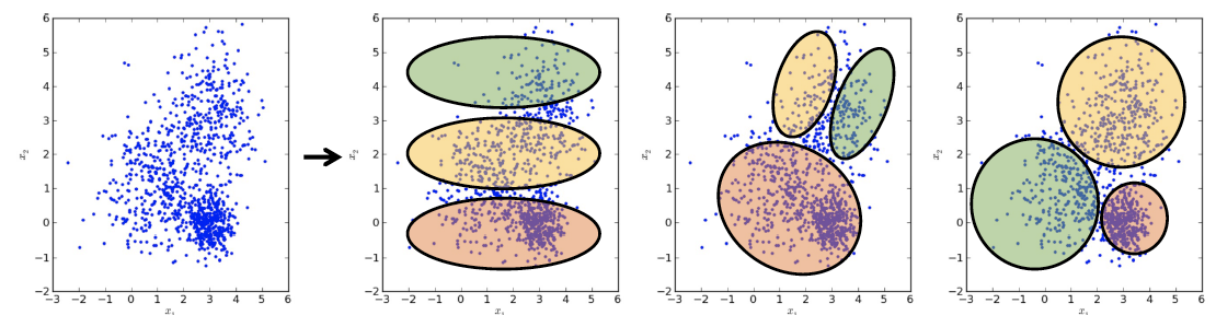
Clustering

Unlabeled data points를 여러 group으로 partitioning하는 것

💡

Partition하는 기준은 similarity 일 수도 있고, distance 일 수도 있다.

Non-parametric approach

K-means clustering

Soft K-means clustering

Parametric approach

Mixture of Gaussian (Generative model로 볼 수도 있음)

💡

GMM을 clustering으로 보겠다는 의미는 여러 multi-gaussian distribution 중 하나로 cluster시킨다는 의미로 이해하면 된다.

Example: Image Segmentation

Image segmentation can be performed by pixel clustering

→ 유사한 특성을 가진 feature들을 clustering하는 것

K-means Algorithm

어느 것이 더 좋은지 판단하기 위해서는 criterion이 필요하다.

💡

K-means Algorithm은 거리 를 기준으로 cluster를 형성하고 싶은 것이다.

이때, $N$개의 data point $\{x_i\}_{i = 1}^N (x_i\in \R^D)$가 있고, 이러한 데이터들을 $K$개의 cluster로 나누려고 한다고 가정하자.

$$\min_{\mu, z} J = \sum_{i = 1}^N\sum_{k = 1}^K z_{ik}\|x_i-\mu_k\|^2 \\ z_{ik}\in \{0, 1\} \forall i, k\text{ and }\sum_{k = 1}^K z_{ik} = 1$$

where $z_i = \{z_{ik}\}_{k = 1}^K$ are the assignment variables for the $i$-th data point. $\mu = \{\mu_k\}_{k = 1}^K$ are the center of $K$ clusters

💡

즉, $z_{ik}$는 대응되는 cluster에만 1을 가진다. 해당하는 cluster에 대해서만, 해당 cluster의 center와의 distance를 구해서 더함.

Procedure

1. $\mu$ 를 랜덤하게 선택한다. (i.e. $K$개의 cluster의 중심을 랜덤으로 설정한다.)

2. Assignment step : Given $\mu$, find the optimal assignment variables $z$

   $$z_{ik} = \begin{cases} 1 & \text{if }k = \argmin_k \|x_i-\mu_k\|^2\\ 0 & \text{otherwise}\end{cases}$$

   💡

   즉 주어진 cluster의 중심으로부터 가장 가까운 cluster에 할당하는 작업이라고 이해해주면 된다.

3. Update step : Given $z$, find the optimal centroids $\mu$

   $$\mu_k = \frac{\sum_{i}z_{ik}x_i}{\sum_iz_{ik}}$$

   💡

   즉, cluster에 속한 것끼리만 평균을 취해서 새로운 centroid를 계산하는 것이다.

   💡

   위 식은 $J$를 $\mu_k$에 대해서 미분하고 0이되는 값을 구한 결과이다.

4. Repeat until converge

   

Always converges?

The cost function is guaranteed to decrease monotonically in each iteration because the data points are always assigned to the closest centroid. This means that the distance between each data point and its assigned centroid is always decreasing. As a result, the cost function, which is the sum of the squared distances between each data point and its assigned centroid, is also guaranteed to decrease monotonically.

→ 귀류법으로 증명할 수 있음

→ 만약에 커진다고 가정하면 모순이 나옴. (애초에 최소가 되게끔하는 방향으로 centroid가 움직이므로)

The K-means algorithm does not always converge to the global minimum because the initial choice of centroids can affect the final clustering. If the initial choice of centroids is not representative of the data, the algorithm may converge to a local minimum that is not the global minimum.

💡

즉 수렴한다고는 항상 보장할 수 있지만, 그게 global optima라고까지는 보장할 수 없다. 따라서 초기값을 어떻게 설정하느냐가 학습의 결과를 결정하는데 굉장히 중요하게 된다.

Properties

1. Local optimum is found

2. Convergence is guaranteed in a finite number of iteration

3. Computational complexity per iteration
   1. Assignment step : $O(KND)$ D는 data의 dimension

      💡

      모든 data $N$개에 대해서, 존재하는 모든 cluster $K$개의 centroid와의 거리를 비교해야하기 때문이다. 추가적으로 data space가 $\R^D$라고 가정해서 추가로 $D$만큼의 시간복잡도가 들어가는 것이다.

   2. Update step : $O(N)$

Limitations

1. 초기 centroid에 민감함

   → 좀 더 이 부분에 robust한 모델이 K-means++

   💡

   앞서 살펴본 것처럼 초기 centroid 설정에 따라서 global optima에 도달할 수 있는 지 여부가 달라지게 된다.

2. Outlier에 민감함

   

   → 좀 더 이 부분에 robust한 모델이 K-medoids (centroids as the actual data points)

   💡

   해당 부분은 과제에 나왔으므로 주의하도록 하자.

3. The shape of each cluster is always convex

   → Convex hull을 그려봤을 때 convex가 그려짐

4. The number of clusters K should be pre-specified (K는 hyper-parameter이다.)

   

   → 좀 더 이 부분에 robust한 모델이 DBSCAN (density-based clustering algorithm)

   💡

   맨 마지막의 경우 DBSCAN의 경우 1개로 cluster되는 문제가 있음. (k-means는 3개로 설정한 경우 강제로 찢을 수 있음)

   💡

   즉 몇 개의 cluster로 나눌 것인지를 학습이 되기 전에 미리 지정해야한다는 문제점이 존재하는 것이다.

Soft K-means Algorithm

$$\min_{\mu, z}J = \sum_{i = 1}^N\sum_{k = 1}^K z_{ik}\|x_i - \mu_k\|^2 + \frac{1}{\beta}\sum_{i = 1}^N\sum_{k = 1}^K z_{ik}\log z_{ik}$$

💡

기존 k-means algorithm과 달리 $z_{ik}$가 0 아니면 1이 아니라 일종의 probability 처럼 사용하자는 것

💡

$-\sum_{k = 1}^K z_{ik}\log z_{ik}$ 는 entropy에 대한 인자이다. 즉 entropy가 작은 것에 대한 penalty를 제공한다고 생각해주면 된다. (Entropy가 클수록 Randomness가 크게 된다.)

💡

$\beta$를 작게할수록 penalty를 크게 부여하는 것이므로 Randomness를 강제한다고 생각해주면 된다. 즉 soft-assignment를 강제하는 효과를 가져온다.