6. Approximation and fitting

Norm approximation

Basic norm approximation problem

Assume that the columns of $A$ are independent.

$$\text{minimize }\|Ax - b\|$$

where $A\in \R^{m\times n}$ with $m\ge n$, $\|\cdot\|$ is a norm of $\R^m$

Geometric interpretation

Geometrically, the solution $x^*$ is the point such that $Ax^*\in \mathcal R(A)$ that closest to $b$. The vector

$$r = Ax - b$$

is called the residual for the problem; its components are sometimes called the individual residuals associated with $x$.

Estimation interpretation

It can be interpreted as a problem of estimating a parameter vector based on an imperfect linear vector measurement. We consider a linear measurement model

$$y = Ax + v$$

where $y\in \R^m$ is a vector measurement, $x\in \R^n$ is a vector of parameters to be estimated, and $v\in \R^m$ is some unknown measurement error, presumed to be small in the norm $\|\cdot\|$. The estimation problem is to make a sensible guess as to what $x$ is for given $y$.

If we guess that $x$ has the value $\hat x$, the most plausible guess for $x$ is

$$\hat x = \argmin_z \|Ax - y\|$$

Example

1. least squares approximation ($\|\cdot \|_2$)

   The most common norm approximation problem involves the Euclidean or $l_2$-norm. By squaring the objective, we obtain an equivalent problem which is called the least-squares approximation problem

   $$\text{minimize }\|Ax-b\|_2^2 = r_1^2 + \cdots + r_m^2$$

   where the objective is the sum of squares of the residuals. It can be solvable by normal equations

   $$A^TAx = A^Tb$$

   If $A$ has a full rank (i.e. the rows of $A$ are independent), the least-squares approximation problem has a unique solution

   $$x = (A^TA)^{-1}A^Tb$$

2. Chebyshev approximation ($\|\cdot \|_\infty$)

   When the $l_\infty$-norm is used, the norm approximation problem

   $$\text{minimize }\|Ax - b\|_\infty = \max\{|r_1|, \dots, |r_m|\}$$

   is called the Chebyshev approximation problem or minimax approximation problem since we are to minimize the maximum absolute value of residuals. The Chebyshev approximation problem can be solved as an LP

   $$\text{minimize }t$$

   subject to

   $$-t\bold1 \preceq Ax - b\preceq t\bold 1$$

   with variables $x\in \R^n$ and $t\in \R$

3. Sum of absolute residuals approximation ($\|\cdot \|_1$)

   When the $l_1$-norm is used, the norm approximation problem

   $$\text{minimize }\|Ax-b\|_1 = |r_1| + \cdots + |r_m|$$

   is called the sum of absolute residuals approximation problem, or in the context of estimation, it is called a robust estimator. Like the Chebyshev approximation problem, this problem can be expressed as an LP

   $$\text{minimize }1^Tt$$

   subject to

   $$-t \preceq Ax - b\preceq t$$

   with variables $x\in \R^n$ and $t\in \R$

Penalty function approximation

In $l_p$-norm approximation, for $1\le p<\infty$, the objective is

$$(|r_1|^p + \cdots + |r_m|^p)^{1/p}$$

As in least-squares problems, we can consider the equivalent problem with objective

$$|r_1|^p + \cdots + |r_m|^p$$

which is a separable and symmetric function of the residuals. In particular, the objective only depends on the amplitude distribution of the residuals (i.e. the residuals in sorted order)

We will consider a useful generalization of the $l_p$-norm approximation problem that only depends on the amplitude distribution of the residuals.

The penalty function approximation problem has the form

$$\text{minimize }\phi(r_1) + \cdots + \phi(r_m)$$

subject to

$$r = Ax - b$$

where $\phi:\R\to \R$ is called the residual penalty function.

💡

We assume that $\phi$ is convex, so the penalty function approximation problem is a convex optimization problem.

💡

By choosing $x$, $r$ is determined. Moreover, the feasible set of $r$ is an affine set.

💡

By using penalty functions, we can give more weight to a specific component.

💡

We can view the penalty function approximation problem as a multi-criterion optimization problem.

Examples

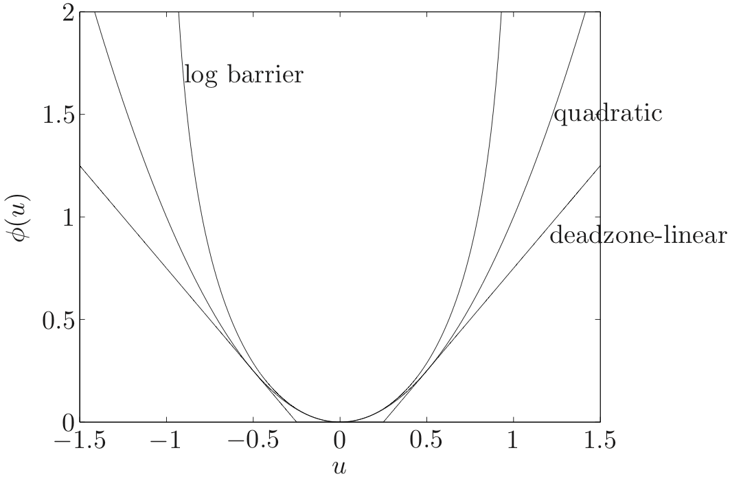
1. quadratic

   $$\phi(u) = u^2$$

   💡

   It is the most typical penalty function because we already know the analytical solution of it.

   💡

   Unlike the L1 norm, the penalty function value increases faster as the residual grows larger.

2. deadzone linear with width $a$

   $$\phi(u) = \text{max\{0, |u|\;-\;a\}}$$

   💡

   Neglect the residual if its values is less than $a$

3. log-barrier with limit $a$

   $$\phi(u) = \begin{cases}-a^2\log(1-(u/a)^2 & |u|<a \\ \infty & \text{otherwise}\end{cases}$$

   💡

   It goes to infinity if a residual located in the outside of the limit.

   💡

   If the residual is small, the penalty function behaves similarly to a quadratic function. However, if the residual is large, its value will increase much more rapidly than that of a quadratic function.

We take a matrix $A\in \R^{100\times 30}$ and vector $b\in \R^{100}$, and compute the $l_1$-norm and $l_2$-norm approximate solutions of $Ax \approx b$, as well as the penalty function approximations with a dead zone linear penalty with $a = 0.5$ and log barrier penalty with $a = 1$. The following figure shows the four associated penalty functions and the amplitude distributions of the optimal residuals for these four penalty approximations.

Histogram of optimal point of r with respect to 4 different penalty functions

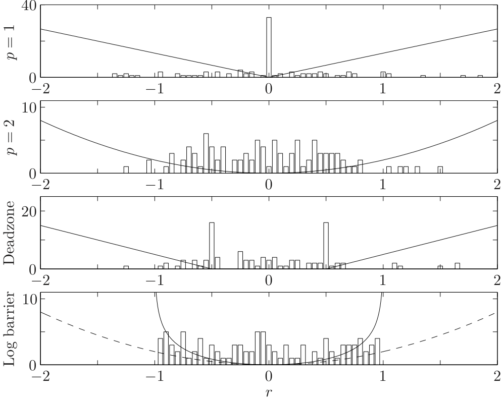
Several features can be derived from the amplitude distributions

1. For the $l_1$-optimal solution, many residuals are either zero or very small. The $l_1$-optimal solution also has relatively larger residuals than the others.

   💡

   Compared to $l_2$-norm, this converges to zero for relatively small residuals due to the higher penalty imposed when the residuals are small.

2. The $l_2$-norm approximation has many modest residuals, and relatively few larger ones.

   💡

   When the residual is small, the value of the penalty value is already small enough so that we can quit the procedure.

3. For the dead zone linear penalty, we see that many residuals have the value $\pm 0.5$, right at the edge of the free zone.

4. For the log barrier penalty, we see that no residuals have a magnitude larger than 1, but otherwise the residual distribution is similar to the residual distribution for $l_2$-norm approximation.

Penalty function approximation with sensitivity to outliers

In the estimation or regression context, an outlier is a measurement $y_i = a_i^Tx + v_i$ for which the noise $v_i$ is relatively large. This is often associated with faculty data or a flawed measurement. When outliers occur, any estimate of $x$ will be associated with a residual vector with some large components.

Ideally, we would like to guess which measurements are outliers, and either remove them from the estimation process or greatly lower their weight in forming the estimate. This could be accomplished using penalty function approximation such as

$$\phi(u) = \begin{cases}u^2 & |u|\le M \\ M^2 & \text{otherwise}\end{cases}$$

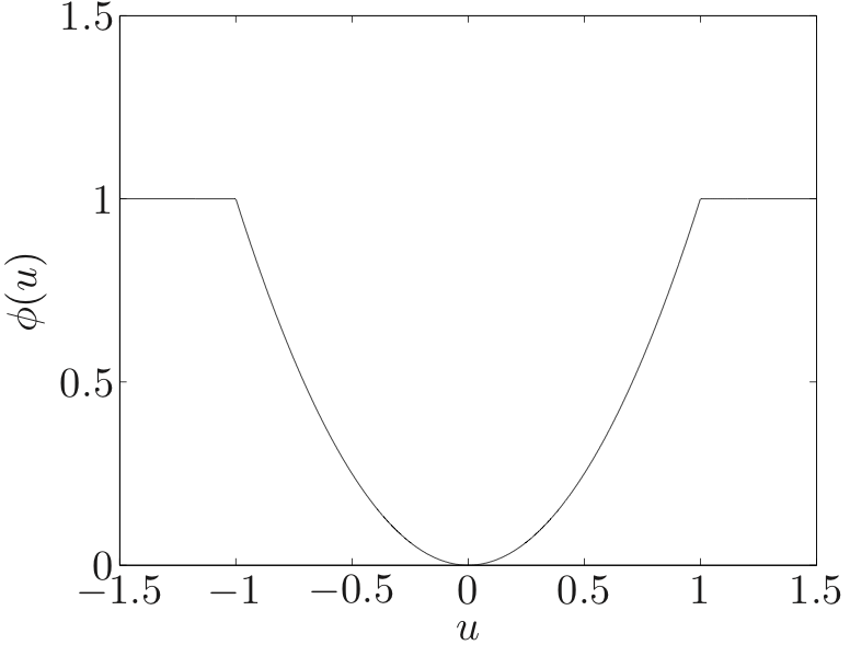
This penalty function agrees with least-squares for any residual smaller than $M$, but puts a fixed weight on any residual larger than $M$, no matter how much larger it is.

💡

By doing so, we can alleviate the impact of the outlier.

The problem is that, like we can see above, it is not a convex function. The sensitivity of a penalty function depends on the value of the penalty function for large residuals. If we restrict ourselves to convex penalty functions, the ones that are least sensitive are those for which $\phi(u)$ grows linearly (like $l_1$-norm).

💡

Penalty functions with this property are sometimes called robust, since the associated penalty function approximation methods are much less sensitive to outliers than least-squares.

One obvious example of a robust penalty function is $\phi(u) = |u|$. Another example is the robust least-squares or Huber penalty function given by

$$\phi_{\text{hub}}(u) = \begin{cases}u^2 & |u| \le M \\ M(2|u|-M) & \text{otherwise}\end{cases}$$

💡

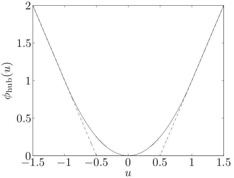
Actually, $M(2|u|-M)$ is a tangent line of the quadratic function at $u = M$ and $-M$

💡

It can be interpreted as a mixture of $l_1$-norm and $l_2$-norm.

💡

Since $l_1$-norm approximation is among the convex penalty function approximation methods that are most robust to outliers. So it is sometimes called robust estimation or robust regression

Least norm problems

The basic least-norm problem has the form

$$\text{minimize }\|x\|$$

subject to

$$Ax = b$$

where the data are $A\in \R^{m\times n}$ with $m\le n$ and $b\in \R^m$, the variable is $x\in \R^n$, and $\|\cdot \|$ is a norm on $\R^n$. Assume that the rows of $A$ are independent.

💡

The least-norm problem is a convex optimization problem

• Geometric interpretation

  $x^*$ is a point in affine set $\{x |\; Ax = b\}$ with minimum distance to 0

• Estimation interpretation

  $b = Ax$ are perfect measurement of $x$. $x^*$ is the smallest estimate consistent with measurements.

  💡

  Assume we don’t have enough measurement to identify a parameter perfectly (the nullity is not zero), but measurements are perfect.

Example

1. Least-squares solution of linear equations ($\|\cdot \|_2$)

   By squaring the objective we obtain the equivalent problem

   $$\text{minimize }\|x\|_2^2$$

   subject to

   $$Ax = b$$

   Like the least-squares approximation problem, this problem can be solved analytically. By introducing the dual variable $\nu\in \R^m$, the optimality conditions are

   $$2x^* + A^T\nu^* = 0 \\ Ax ^* = b$$

   Then

   $$\nu^* = -2(AA^T)^{-1}b \\ x^* = A^T(AA^T)^{-1}b$$

   💡

   Since $\text{rank }A = m < n$, the matrix $AA^T$ is invertible

2. Sparse solutions via least $l_1$-norm

   $l_1$-norm approximation gives relatively large weight to small residuals so that it produces a solution $x$ with a large number of components equal to zero.

   💡

   $l_1$-norm problem tens to produce sparse solutions of $Ax = b$

3. Least penalty problem

   $$\text{minimize }\phi(x_1) + \cdots + \phi(x_n)$$

   subject to

   $$Ax = b$$

   where $\phi:\R\to \R$ is a convex penalty function.

Regularized approximation

The goal is to find a vector $x$ that is small, and also makes the residual $Ax - b$ small. This is naturally described as a convex vector optimization problem with two objectives.

$$\text{minimize (w.r.t }R_+^2) \; (\|Ax-b\|, \|x\|)$$

where $A\in \R^{m\times n}$ and norms on $\R^m$ and $\R^n$ can be different.

💡

We want to find a good approximation $Ax \approx b$ with small $x$

Regularization

Regularization is a common scalarization method used to solve the bi-criterion problem. One form of regularization is to minimize the weighted sum of the objectives

$$\text{minimize }\|Ax -b \| + \gamma \|x\|$$

where $\gamma >0$ is a problem parameter.

Another common method of regularization is to minimize the weighted sum of squared norms

$$\text{minimize }\|Ax - b\|^2 + \delta \|x\|^2$$

The most common form of regularization is

$$\text{minimize }\|Ax-b\|_2^2 + \delta \|x\|_2^2$$

It is called Tikhonov regularization. It has the analytical solution

$$x = (A^TA+\delta I)^{-1}A^Tb$$

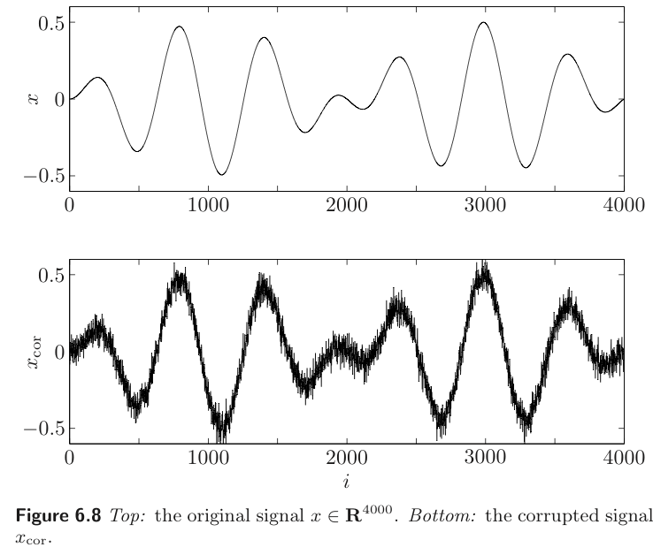
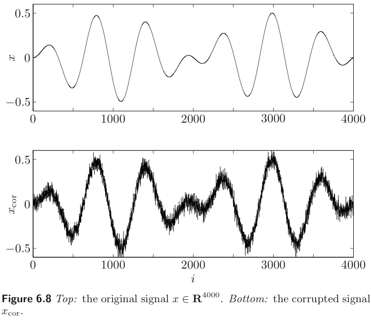
Signal reconstruction

In reconstruction problems, we start with a signal represented by a vector $x\in \R^n$. The coefficients $x_i$ correspond to the value of some function of time, evaluated at evenly spaced points.

💡

It is usually assumed that the signal doesn’t vary too rapidly. (i.e. We have $x_i\approx x_{i + 1}$)

The signal $x$ is corrupted by an additive noise $v$

$$x_{cor} = x + v$$

The goal is to form an estimate $\hat x$ of the original signal $x$, given the corrupted signal $x_{cor}$. This process is called signal reconstruction.

💡

It is related to the denoising process. Moreover, most reconstruction methods end up performing some sort of smoothing operation on $x_{cor}$ to produce $\hat x$, so it is also called smoothing

One simple formulation of the reconstruction problem is the bi-criterion problem

$$\text{minimize (w.r.t }\R_{+}^2) \; (\|\hat x - x_{cor}\|, \phi(\hat x))$$

where $\phi:\R^n\to \R$ is convex, and it is called regularization function or smoothing objective.

💡

It is meant to measure the roughness, or lack or smoothness, of the estimate $\hat x$.

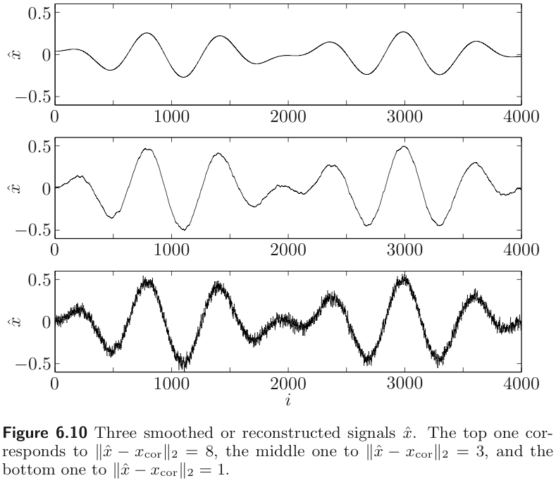
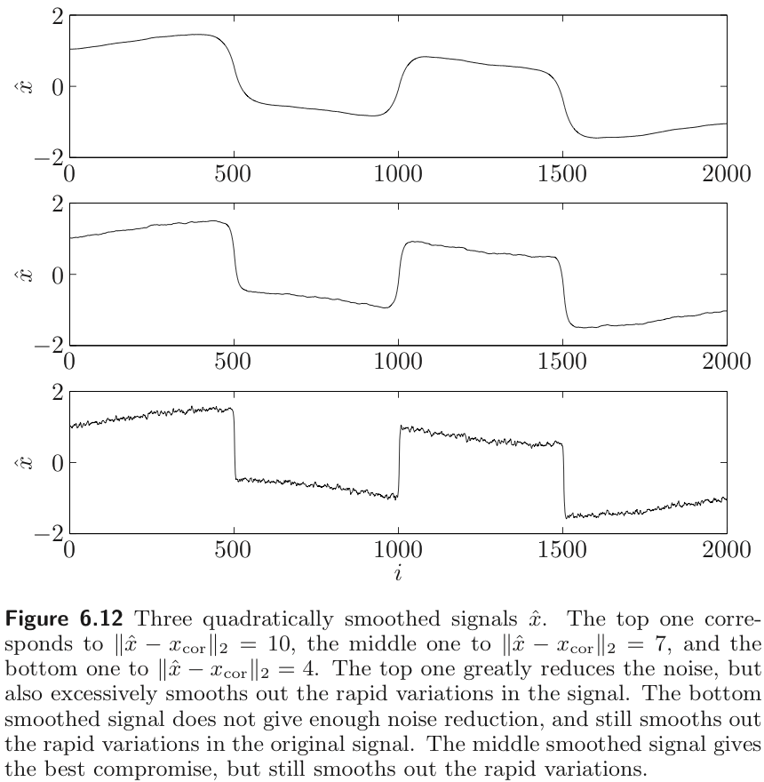
Example : Quadratic smoothing

The simplest reconstruction method uses the quadratic smoothing function

$$\phi_{quad}(x) = \sum_{i = 1}^{n - 1}(x_{i + 1} - x_i)^2 =\|Dx\|_2^2$$

where $D\in \R^{(n - 1)\times n}$ is the bidiagonal matrix.

$$D = \begin{bmatrix}-1 & 1 & 0 & \cdots & 0 & 0 & 0 \\ 0 & -1 & 1 & \cdots & 0 & 0 & 0 \\ \vdots & \vdots & \vdots & & \vdots & \vdots & \vdots \\ 0 & 0 & 0 & \cdots & -1 & 1 & 0 \\ 0 & 0 & 0 & \cdots & 0 & -1 & 1\end{bmatrix}$$

We can obtain the optimal trade-off between $\|\hat x - x_{cor}\|_2$ and $\|D\hat x\|_2$ by minimizing

$$\|\hat x - x_{cor}\|_2^2 + \delta \|D\hat x\|_2^2$$

where $\delta >0$ parameters the optimal trade-off curve.

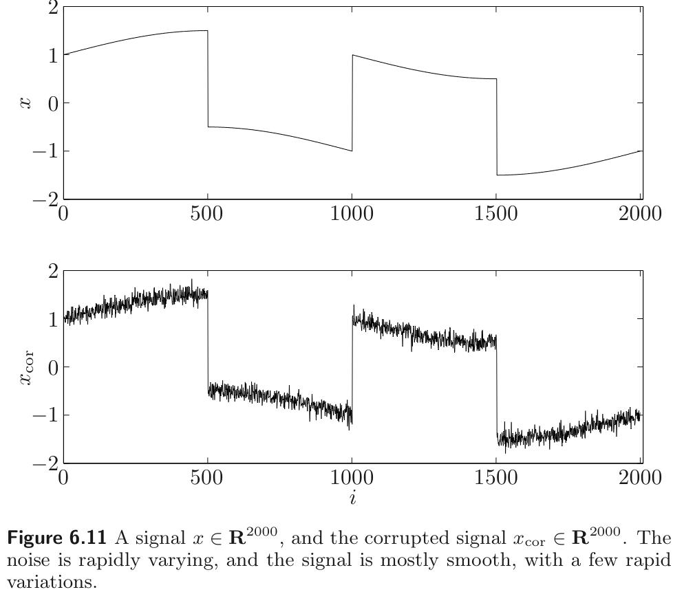
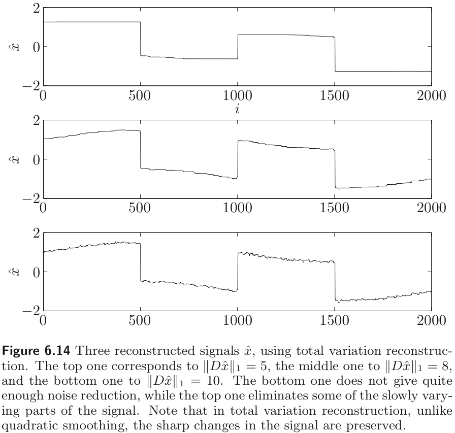
Example : Total variation reconstruction

Simple quadratic smoothing works well as a reconstruction method when the original signal is very smooth, and the noise is rapidly varying. But any rapid variations in the original signal will be removed by quadratic smoothing.

Total variation reconstruction method can remove much of the noise, while still preserving rapid variations in the original signal. The method is based on the smoothing funciton

$$\phi_{tv}(\hat x) = \sum_{i = 1}^{n - 1}|\hat x_{i + 1}- \hat x_i| = \|D\hat x\|_1$$

💡

Similar to $l_1$-norm, it gives less penalty for rapid variation than the quadratic one.

Therefore, we have to choose the smoothing objective carefully regarding of the characteristic of the noise and signal.

💡

quadratic smoothing smooths out noise and sharp transition signal

💡

total variation smoothing preserves sharp transitions in signal because $l_1$-norm has less sensitive for the large value than $l_2$-norm.

Robust approximation

We consider an approximation problem with basic objective $\|Ax - b\|$, but also wish to take into account some uncertainty or possible variation in the data matrix $A$. There are two approches to solve this problem.

1. stochastic : assume $A$ is random and minimize $\mathbb E (\|Ax-b\|)$

2. worst-case : set $\mathcal A$ of possible values of $A$ and minimize $\sup_{A\in \mathcal A}\|Ax - b\|$

Stochastic robust approximation

We assume that $A$ is a random variable taking values in $\R^{m\times n}$, with mean $\bar A$. Then

$$A= \bar A + U$$

where $U$ is a random matrix with zero mean.

It is natural to use the expected value of $\|Ax - b\|$ as the objective

$$\text{minimize }\mathbb E(\|Ax - b\|)$$

We refer to this problem as the stochastic robust approximation problem.

💡

It is always a convex optimization problem, but usually not tractable.

Worst-case robust approximation

It is also possible to model the variation in the matrix $A$ using a worst case approach. We describe the uncertainty by a set of possible values for $A$

$$A\in \mathcal A\sub \R^{m\times n}$$

which we assume is non-empty and bounded. We define the associated worst-case error of a candidate approximate solution $x\in \R^n$ as

$$e_{wc}(x) = \sup_{A\in \mathcal A}\|Ax - b\|$$

which is always a convex function of $x$.

💡

It is a convex function because it is just a point-wise supremum which is always convex.

The worst-case robust approximation problem is to minimize the worst case error

$$\text{minimize }e_{wc}(x) = \sup_{A\in \mathcal A}\|Ax - b\|$$

where the variable is $x$, and the problem data are $b$ and the set $\mathcal A$.

💡

When $\mathcal A$ is the singleton, the robust approximation problem reduces to the basic norm approximation problem.

It is always a convex optimization problem, but its tractability depends on the norm used and the description of uncertainty of $\mathcal A$.

Example

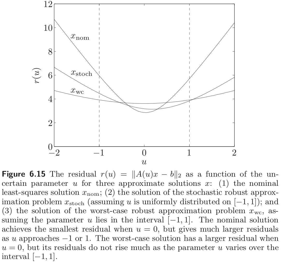
To illustrate the difference between the stochastic and worst-case formulations for the robust approximation problem, we consider the least squares problem

$$\text{minimize }\|A(u)x - b\|_2^2$$

where $u\in \R$ is an uncertain parameter and $A(u) = A_0 + uA_1$. We consider a specific instance of the problem, with $A(u)\in \R^{20\times 10}$, $\|A_0\| = 10, \|A_1\| = 1$, and $u$ in the interval $[-1, 1]$.

We find three approximate solutions

1. Nominal optimal : The optimal solution $x_{nom}$ is found, which minimize $\|A_0x - b\|_2^2$

2. Stochastic robust approximation : We find $x_{stoch}$, which minimizes $\mathbb E(\|A(u) x - b\|_2^2$, assuming the parameter $u$ is uniformly distributed on $[-1, 1]$

3. Worst-case robust approximation. We find $x_{wc}$, which minimizes

   $$\sup_{-1\le u\le 1}\|A(u)x - b\|_2$$

Example : stochastic robust Least squares

Consider the stochastic robust least-squares problem

$$\text{minimize }\|Ax - b\|_2^2$$

where $A = \bar A + U$, $U$ is a random matrix with zero mean.

We can express the objective as

$$\begin{aligned}\mathbb E(\|Ax - b\|_2^2) &= \mathbb E\bigg((\bar Ax -b+Ux)^T(\bar Ax -b+Ux)\bigg) \\ &= (\bar A x - b)^T(\bar Ax-b) + \mathbb E(x^TU^TUx) \\ &=\|\bar Ax-b\|_2^2 + x^TPx\end{aligned}$$

where $P = \mathbb E(U^TU)$

Therefore, the stochastic robust approximation problem has the form of regularized least-squares problem

$$\text{minimize }\|\bar Ax - b\|_2^2 + \|P^{1/2}x\|_2^2$$

with solution

$$x= (\bar A^T\bar A+P)^{-1}\bar A^Tb$$

When the matrix $A$ is subject to variation, the vector $Ax$ will have more variation the laarger $x$ is, and Jensen’s inequality tells us that variation in $Ax$ will increase the average value of $\|Ax - b\|_2$. So we need to balance making $\bar Ax -b$ small with the desire for a small $x$ to keep the variation in $Ax$ small.

For $P = \delta I$, we can get Tikhonov regularized least squares problem

$$\text{minimize }\|\bar Ax - b\|_2^2 + \delta \|x\|_2^2$$

💡

Therefore, regularized least squares problem can be interpreted as a stochastic concept and vice versa.

Example : worst case robust least squares

Let

$$\mathcal A = \{\bar A + u_1 A_1 + \cdots + u_pA_p|\; \|u\|_2 \le 1\}$$

Consider the worst case robust least-squares problem

$$\text{minimize }\sup_{A\in \mathcal A}\|Ax - b\|_2^2 = \sup_{\|u\|_2\le 1} \|P(x)u + q(x)\|_2^2$$

where $P(x) = \begin{bmatrix}A_1x & A_2x & \cdots & A_px\end{bmatrix}, q(x) = \bar Ax -b$

Note that the strong duality holds between the following problems

1. Primal problem

   $$\text{maximize }\|Pu+ q\|_2^2$$

   subject to

   $$\|u\|_2^2\le 1$$

   💡

   Intuitively, we can solve this problem by finding a maximum singular value.

2. Dual problem

   $$\text{minimize }t+ \lambda$$

   subject to

   $$\begin{bmatrix}I & P & q \\P^T & \lambda I & 0 \\ q^T & 0 & t\end{bmatrix}\succeq 0$$

💡

It is a very specially case of satisfying the strong duality condition when the problem is not a convex.

Therefore, the Lagrange dual of this problem can be expressed as the SDP

$$\text{minimize }t+ \lambda$$

subject to

$$\begin{bmatrix}I & P(x) & q(x) \\P(x)^T & \lambda I & 0 \\ q(x)^T & 0 & t\end{bmatrix}\succeq 0$$

with variables $t, \lambda\in \R$.

For fixed $x$, we can compute $\sup_{\|u\|_2\le 1} \|P(x)u + q(x)\|_2^2$ by solving the SDP with variables $t$ and $\lambda$. In other words, optimizing jointly over $t, \lambda$, and $x$ is equivalent to minimizing worst case error $e_{wc}(x)^2$.

💡

Therefore, the robust least squares problem is equivalent to the SDP with $x, \lambda , t$ as variables.