4. Convex optimization problems

Optimization problem in standard form

$$\text{minimize } f_0(x)$$

subject to

$$f_i(x) \le 0, \; i = 1, \dots, m \\ h_i(x) = 0, \; i = 1, \dots, p$$

• $x\in \R^n$ is the optimization variable

• $f_0:\R^n\to \R$ is the objective or cost function

• $f_i:\R^n\to \R, \; i = 1, \dots, m$ are the inequality constraint functions

• $h_i:\R^n\to \R, \; i = 1, \dots, p$ are the inequality constraint functions

Optimal value

$$p^* = \inf\{f_o(x) |\; f_i(x)\le 0, \; i = 1, \dots, m, h_i(x) = 0, \; i = 1, \dots, p\}$$

1. $p^* = \infty$ if a problem is infeasible (no $x$ satisfies the constraints)

2. $p^* = -\infty$ if a problem is unbounded below

Optimal and locally optimal points

• $x$ is feasible if $x\in \text{dom }f_0$ and it satisfies all constraints

• a feasible $x$ is optimal $f_0(x) = p^*$; $X_{opt}$ is the set of optimal points

• $x$ is locally optimal if there is an $R>0$ such that $x$ is optimal for

  $$\text{minimize } f_0(z)$$

  subject to

  $$f_i(z) \le 0, \; i = 1, \dots, m \\ h_i(z) = 0, \; i = 1, \dots, p \\ \|z -x\|_2\le R$$

  💡

  It can be interpreted as the restricted domain of $f_0$

Examples

• $f_0(x) = 1/x, \text{dom }f_0 = \R_{++}$ : $p^* = 0$, but it has no optimal point.

  💡

  We have to distinguish between optimal point and optimal value

• $f_0(x) = -\log x, \text{dom }f_0 = \R_{++}$: $p^* = -\infty$

Implicit constraints

the standard form optimization problem has an implicit constraint

$$x\in \mathcal D = \bigcap_{i = 0}^m\text{dom }f_i \cap \bigcap_{i = 1}^p\text{dom }h_i$$

we call $\mathcal D$ the domain of the problem.

Feasibility problem

$$\text{find }x$$

subject to

$$f_i(x) \le 0, \; i = 1, \dots, m \\ h_i(x) = 0, \; i = 1, \dots, p$$

can be considered a special case of the general problem with $f_0(x) = 0$

Convex optimization problem

$$\text{minimize }f_0(x)$$

subject to

$$f_i(x) \le 0, \; i = 1, \dots, m \\ h_i(x) = 0, \; i = 1, \dots, p$$

• $f_0, \dots, f_m$ are convex, $h_1, \dots, h_p$ are affine

• problem is quasi-convex if $f_0$ is quasi-convex and $f_1, \dots, f_m$ convex

often written as

$$\text{minimize }f_0(x)$$

subject to

$$f_i(x) \le 0, \; i = 1, \dots, m \\ Ax = b$$

💡

feasible set of a convex optimization problem is a convex set

💡

The convex optimization problem is not an attribute of the feasible set. It is an attribute of the problem description.

• equivalent problem : by solving one, we can construct the other solution

• identical problem : objective and constraints are identical

Local and global optima

any locally optimal point of a convex problem is globally optimal

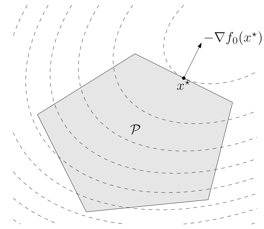
Optimality criterion for differentiable objective function

Suppose that the objective $f_0$ in a convex optimization problem is differentiable, so that for all $x, y\in \text{dom }f_0$,

$$f_0(y) \ge f_0(x) + \nabla f_0(x)^T(y-x)$$

Then $x$ is optimal if and only if it is feasible and

$$\nabla f_0(x)^T(y-x)\ge 0$$

for all feasible $y$

• Proof

  We already know that $f_0(y) \ge f_0(x) + \nabla f_0(x)^T(y-x)$

  If $\nabla f_0(x)^T(y- x) \ge 0$ for all feasible $y$, then $f_0(y) \ge f_0(x)$ for all feasible $y$. Therefore, $x$ is optimal.

  Conversely, suppose $x$ is optimal and there exists $y$ is feasible region such that

  $$\nabla f_0(x)^T(y-x) < 0$$

  That means $y$ is located in the half-space that corresponds to the negative sign of the $\nabla f_0(x)$. It contradicts the assumption.

  Therefore, $\nabla f_0(x)^T(y-x) \ge 0$ for all $y$ in the feasible region.

💡

if non-zero, $\nabla f_0(x)$ defines a supporting hyperplane to a feasible set $X$ at $x$

• unconstrained problem : $x$ is optimal if and only if

  $$x\in \text{dom }f _0\quad \nabla f_0(x) = 0$$

  💡

  In an unconstrained problem case, we can put arbitrary $y$ so the only option that we can choose is $\nabla f_0(x) = 0$

• equality constrained problem

  $$\text{minimize }f_0(x)$$

  subject to

  $$Ax = b$$

  (Assume that it is non-empty; otherwise the problem is unfeasible)

  $x$ is optimal if and only if there exists a $\nu$ such that

  $$x\in \text{dom }f_0 \quad Ax = b \quad \nabla f_0(x) + A^T\nu = 0$$

  • Proof

    Since $x, y$ is in the feasible region,

    $$Ax = b \text{ and }Ay = b$$

    That means

    $$x- y \in \mathcal N(A)$$

    Therefore, the first optimality condition can be written as

    $$\nabla f_0(x)^Tz\ge 0, \forall z\in \mathcal N(A)$$

    Since $\mathcal N(A)$ is a subspace,

    $$\nabla f_0(x)^T(-z) \ge 0, \forall \in \mathcal N(A)$$

    That means

    $$\nabla f_0(x)^Tz = 0 , \forall z\in \mathcal N(A)$$

    So,

    $$\nabla f_0(x) \perp \mathcal N(A)$$

    Since $\mathcal N(A) \perp \mathcal R(A^T)$, (equivalently, $\mathcal R(A^T)$ is row space of $A$)

    

    3F theorem (Linear algebra and its application written by Gilbert Strang)

    $$\nabla f_0(x) \in \mathcal R(A^T) \\ \Rightarrow \exists v\in \text{dom }A, \nabla f_0(x) = A^Tv$$

    Since $\text{dom }A$ is a vector space, it is equivalent to say that

    $$\exist v\in \text{dom }A, \nabla f_0(x) + A^Tv = 0$$

  💡

  This is the classical Lagrange multiplier optimality condition

• minimization over nonnegative orthant

  $$\text{minimize }f_0(x)$$

  subject to

  $$x\succeq 0$$

  $x$ is optimal if and only if

  $$x\in \text{dom }f_0 \quad x\succeq 0 \quad \begin{cases}\nabla f_0(x)_i \ge 0 & x_i = 0 \\ \nabla f_0(x)_i = 0 & x_i > 0 \end{cases}$$

  • Proof

    The first order optimality condition is

    $$\nabla f_0(x)^T(y-x)\ge 0$$

    for all feasible $y$

    Since $y$ is in the feasible region, $y\succeq 0$. So $\nabla f_0(x)\succeq 0$, it not $\nabla f_0(x)^Ty$ is not unbounded below. Then $\nabla f_0(x)^Ty \ge 0$ for all feasible $y$.

    Therefore

    $$- \nabla f_0(x)^Tx \ge 0$$

    Since $\nabla f_0(x) \succeq 0, x\succeq 0$,

    $$\begin{cases}\nabla f_0(x)_i \ge 0 & x_i = 0 \\ \nabla f_0(x)_i = 0 & x_i > 0 \end{cases}$$

Equivalent convex problems

two problems are (informally) equivalent if the solution of one is readily obtained from the solution of the other, and vice-versa

some common transformations that preserve convexity

Eliminating equality constraints

$$\text{minimize }f_0(x)$$

subject to

$$f_i(x) \le 0, \quad i = 1, \dots, m \\ Ax = b$$

is equivalent to

$$\text{minimize }_z f_0(Fz+x_0)$$

subject to

$$f_i(Fz + x_0) \le 0 \quad i = 1, \dots, m$$

where $F$ and $x_0$ are such that

$$Ax = b\Leftrightarrow x = Fz + x_0\text{ for some }z$$

Actually let $y$ is in the feasible region (i.e. $Ay = b$ and $f_i(y)\le 0, \forall i$)

$$Ax = b, Ay = b\\\Rightarrow x - y\in \mathcal N(A)$$

Let $\mathcal N$ is a matrix which its columns is the linearly independent vector in $\mathcal N(A)$

💡

However, this problem requires at least one feasible point $x_0$

💡

If the original problem is a convex problem, the transformed problem is also a convex problem since it is just the composition of the affine function.

Introducing equality constraints

$$\text{minimize }f_0(A_0x + b_0)$$

subject to

$$f_i(A_ix + b_i) \le 0, \quad i = 1, \dots, m$$

is equivalent to

$$\text{minimize }_{x, y_i}f_0(y_0)$$

subject to

$$f_i(y_i)\le 0, \quad i = 1, \dots, m\\y_i = A_ix + b_i, \quad i = 1, \dots, m$$

💡

Since this approach eventually increases the number of constraints, there is no progress at first glance. However, this approach can lead to significant progress.

Introducing slack variables for linear inequalities

$$\text{minimize }f_0(x)$$

subject to

$$a_i^Tx \le b_i \quad i = 1, \dots, m$$

is equivalent to

$$\text{minimize }_{x, s}f_0(x)$$

subject to

$$a_i^Tx + s_i = b_i, \quad i = 1, \dots, m \\ s_i \ge 0 \quad i = 1, \dots, m$$

💡

This approach can be applicable when we solve the linear programming problem.

Epigraph form

standard form convex problem is equivalent to

$$\text{minimize }_{x, t}t$$

subject to

$$f_0(x) - t\le 0\\f_i(x)\le 0, \quad i = 1, \dots, m\\ Ax = b$$

💡

By using this, we can change our objective function as a linear objective.

Minimizing over some variables

$$\text{minimize }f_0(x_1, x_2)$$

subject to

$$f_i(x_1) \le 0 \quad i = 1, \dots, m$$

is equivalent to

$$\text{minimize }\bar f_0(x_1)$$

subject to

$$f_i(x_1) \le 0 \quad i = 1, \dots, m$$

where $\bar f_0(x_1) = \inf_{x_2}f_0(x_1, x_2)$

💡

We already know that $\bar f_0$ is a convex function.

💡

Dynamic programming preserves the convexity of the problem.

Quasi-convex optimization

$$\text{minimize }f_0(x)$$

subject to

$$f_i(x) \le 0, \quad i = 1, \dots, m\\Ax = b$$

with $f_0:\R^n\to \R$ quasi-convex, $f_1, \dots, f_m$ convex.

Unlike the convex optimization case, it can have locally optimal points that are not globally optimal.

Nevertheless, a variation of the first-order optimality condition does hold for quasi-convex optimization problems with differentiable objective functions.

In quasi-convex optimization problem, $x$ is optimal if

$$x\in X, \quad \nabla f_0(x)^T(y- x) > 0, \forall y\in X \setminus \{x\}$$

💡

Unlike the convex optimization case, it is only sufficient for optimality.

Representation via a family of convex functions

It will be convenient to represent the sublevel sets of a quasi-convex function $f$ via inequalities of convex functions. We seek a family of convex functions $\phi_t$ such that

$$f_0(x) \le t\Leftrightarrow \phi_t(x) \le 0$$

Evidently $\phi_t$ must satisfy the property that for all $x\in \R^n$,

$$\phi_s(x) \le 0 \Rightarrow \phi_t(x) \le 0$$

for $s\ge t$. This is satisfied if for each $x$, $\phi_t(x)$ is a non-increasing function of $t$ (i.e. $\phi_s(x) \le \phi_t(x)$ whenever $s\ge t$.

If we take

$$\phi_t(x) = \begin{cases}0 & f(x) \le t \\ \infty &\text{otherwise}\end{cases}$$

it satisfies the above conditions.

💡

We call it the indicator function of the t-sublevel of $f$

Note that this representation is not unique, for example, if the sublevel sets of $f$ are closed, we can take

$$\begin{aligned}\phi_t(x) &= \text{dist}(x, \{z|f(z) \le t\}) \\ &= \sup_z\{d(z, x) | \; f(z) \le t\}\end{aligned}$$

Example

$$f_0(x) = \frac{p(x)}{q(x)}$$

with $p$ convex, $q$ concave, and $p(x) \ge 0, q(x) > 0$ on $\text{dom }f_0$ can take $\phi_t(x) = p(x) - tq(x)$

1. for $t\ge 0, \phi_t$ convex in $x$

2. $p(x)/q(x) \le t$ if and only if $\phi_t(x) \le 0$

Quasi-convex optimization via convex feasibility problems

Let $\phi_t:\R^n\to \R, t\in \R$ be a family of convex functions that satisfy

$$f_0(x) \le t \Leftrightarrow \phi_t(x) \le 0$$

and also, for each $x$, $\phi_t(x)$ is a non-increasing function of $t$, i.e.

$$s \ge t \Rightarrow \phi_s(x) \le \phi_t(x)$$

Let $p^*$ is the optimal value of the quasi-convex optimization problem.

If the feasibility problem

$$\text{find }x$$

subject to

$$\phi_t(x) \le 0 \\ f_i(x) \le 0, \quad i = 1, \dots, m \\ Ax = b$$

is feasible, then we have $p^*\le t$. Conversely, if the problem is infeasible, then we can conclude $p^*\ge t$.

💡

Note that we want to find the minimum $t$ such that satisfy the above feasibility problem. Since $\phi_t(x)$ is a non-increasing of $t$, if $t$ satisfy the feasibility for $s\ge t$, $s$ is also satisfy the feasibility.

💡

Note that the above problem is a convex feasibility problem, since the inequality constraint functions are all convex, and the equality constraints are linear.

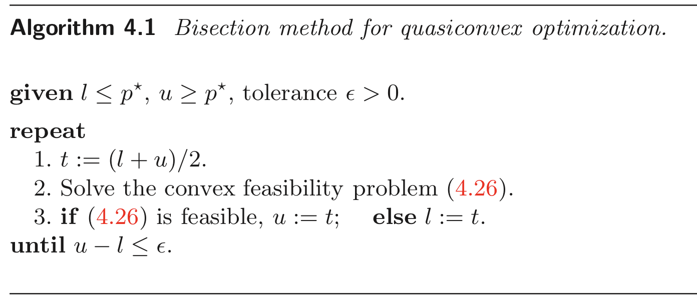
This can be used as the basis of a simple algorithm for solving the quasi-convex optimization problem using bisection (solving a convex feasibility problem at each step)

Assume that the problem is feasible, and start with an interval $[l, u]$ known to contain the optimal value $p^*$. When then solve the convex feasibility problem at its midpoint $t = (l+u) /2$, to determine wheter the optimal value is in the lower or upper half of the interval, and update the interval accordingly. This produces a new interval, which also contains the optimal value, but has half the width of the initial interval.

Basically, the idea is same as the parametric search algorithm.

The blue area in the above figure represents the range of t that satisfies feasibility.

Canonical Problems

Depending on the types of objective function and constraints, optimization problems can be categorized. We will delve into the following six subcategories

• Linear Programming (LP)

• Quadratic Programming (QP)

• Quadratically Constrained Quadratic Programming (QCQP)

• Second-Order Cone Programming (SOCP)

• Semidefinite Programming (SDP)

• Conic Programming (CP)

The above problems have the following inclusion relationships, and moving to the right, they can be seen as more generalized forms.

$$LP\subset QP\subset QCQP\subset SOCP\subset SDP\subset CP$$

Linear program (LP)

$$\text{minimize }c^Tx + d$$

subject to

$$Gx\preceq h \\ Ax = b$$

• Convex problem with affine objective and constraint functions (everything in a linear programming is affine)

• feasible set is a polyhedron

  

💡

Note that the level set of the objective function is just a hyperplane.

But be cautious, as it is not as simple as it might think at first glance because the number of vertices will increase exponentially.

Examples

Piecewise-linear minimization

$$\text{minimize }_x\max_{i = 1, \dots, m}a_i^Tx + b$$

equivalent to an LP

$$\text{minimize }t$$

subject to

$$a_i^Tx + b_i \le t \quad i = 1, \dots, m$$

💡

Actually it is just a epigraph form.

Piecewise linear function

In mathematics and statistics, a piecewise linear, PL or segmented function is a real-valued function of a real variable, whose graph is composed of straight-line segments.&#91;1&#93;

https://en.wikipedia.org/wiki/Piecewise_linear_function

Chebyshev center of a polyhedron

Chebyshev center of

$$\mathcal P = \{x|\; a_i^Tx\le b_i, \; i = 1, \dots, m\}$$

is center of largest inscribed ball

$$\mathcal B = \{x_c + u|\; \|u\|_2 \le r\}$$

$a_i^Tx\le b_i$ for all $x\in \mathcal B$ if and only if

$$\sup\{x_i^T(x_c + u)|\; \|u\|_2\le r\} = a_i^Ts_c + r\|a_i\|_2 \le b_i$$

💡

It is linear in $s_c$ and $r$

Hence $x_c, r$ can be determined by solving the LP

$$\text{maximize }r$$

subject to

$$a_i^Tx_c + r\|a_i\|_2\le b_i \quad i = 1, \dots , m$$

Linear-fractional program

$$\text{minimize }f_0(x)$$

subject to

$$Gx\preceq h \\ Ax = b$$

where

$$f_0(x) = \frac{c^Tx + d}{e^Tx + f} \quad \text{dom }f_0(x) = \{x| \; e^Tx + f > 0\}$$

💡

We already know that linear fractional function is a quasi-convex function

It can be solved by bisection like this

$$f_0(x) \le t \Leftrightarrow c^Tx + d \le t(e^Tx + f)$$

If the feasible set is non-empty, the linear-fractional program can be transformed to an equivalent linear program

$$\text{minimize } c^Ty + dz$$

subject to

$$Gy\preceq hz \\ Ay = bz \\ e^Ty + fz = 1 \\ z \ge 0$$

with variables $y, z$

• Proof

  If $x$ is feasible in our original problem, then

  $$y = \frac{x}{e^Tx +f}, \quad z = \frac{1}{e^Tx + f}$$

  is feasible in the LP problem, with the same objective value $c^Ty + dz = f_0(x)$. Therefore the optimal value of the original problem is greater than or equal to the optimal value of the LP problem. It is has a $y, z$ corresponds to the optimal point of the original problem.

  Conversely,

  1. if $(y, z)$ is feasible in the LP problem with $z\ne 0$, then $x = y/z$ is feasible in the original problem.

  2. If $(y,z)$ is feasible in the LP problem with $z = 0$ and $x_0$ is feasible for the original problem. Then $x = x_0 + ty$ is feasible in the original problem for all $t\ge 0$. Moreover, $\lim{t\to \infty}f_0(x_0 + ty) = c^Ty + dz$, so we can find feasible points in the original function with objective values arbitrarily close to the objective value of $(y, z)$

  💡

  The basic idea is that if we add the additional variable $z$, we can normalize it by using $x$ and $z$. Therefore we can eliminate the denominator. So if $z$ is positive, we can think it as a normalization.

  💡

  If $z = 0$, we can arbitrary add $y$ to $x_0$. This is a main idea to prove above.

Generalized linear-fractional program

$$f_0(x) = \max_{i = 1, \dots, r} \frac{c_i^Tx + d_i}{e_i^Tx + f_j}$$

where $\text{dom }f_0(x) = \{x|\; e_i^Tx + f_i > 0, \; i = 1, \dots, r\}$

a quasi-convex optimization problem. Unlike the linear fractional problem, there is no way to directly convert to LP. However, since it is a quasi-convex problem, it can be solved by bisection.

💡

The sublevel set is just the intersection of sublevel sets which is convex. Therefore, the objective function is a quasi-convex function.

Quadratic program (QP)

The convex optimization problem is called a quadratic program(QP) if the objective function is convex quadratic, and the constraint functions are affine.

$$\text{minimize }\frac{1}{2}x^TPx + q^Tx + r$$

subject to

$$Gx\preceq h \\ Ax = b$$

where $P\in S_{+}^n, G\in \R^{m\times n}$ and $A \in \R^{p\times n}$

In a quadratic program, we minimize a convex quadratic function over a polyhedron.

Note that if $P\in S_{++}^n$, a sublevel set is a elipsoid

• Proof

  Since $P$ is symmetric and positive definite matrix, it has a orthonomal eigenvector. Let say eigenvectors $\{v_1, \dots, v_n\}$, and eigenvalue $\{\lambda_1, \dots, \lambda_n\}$.

  $$\{x|\; f(x) \le \alpha\} = \{x|\; \frac{1}{2}x^TPx + q^Tx + r\le \alpha\}$$

  Let $x = x_1 v_1 + \cdots + x_nv_n$

  $$\begin{aligned}\{x|\; f(x) \le \alpha\} &= \{ x|\; \frac{1}{2}(\lambda_1\|v_1\|x_1^2 + \cdots + \lambda_n\|v_n\|x_n^2 + q_1x_1 + \cdots + q_nx_n + r)\le \alpha\} \\ &= \{x|\frac{1}{2}((\lambda_1\|v_1 \|x_1^2 + q_1x_1) + \cdots + (\lambda_n \|v_n\|x_n^2 + q_nx_n)) \le \alpha - r\} \end{aligned}$$

  Therefore, it is a ellipsoid if it is not a empty set.

💡

If $P$ is not a positive semi-definite (i.e. it has a negative eigenvalue), the problem is belongs to NP hard.

Quadratically constrained quadratic program (QCQP)

$$\text{minimize }\frac{1}{2}x^TP_0x + q_0^Tx + r_0$$

subject to

$$\frac{1}{2}x^TP_i x + q_i^Tx + r_i \le 0, \quad i = 1, \dots, m \\ Ax = b$$

where $P_i\in S_{+}^n$.

If $P_1, \dots, P_m\in S_{++}^n$, the feasible region is a intersection of $m$ ellipsoids and an affine set.

Examples

Lest-squares

We already know that

$$\|Ax - b\|_2^2 = x^TA^TAx - 2b^TAx + b^Tb$$

and since

$$\begin{aligned}x^TA^TAx &= (Ax)^T(Ax) \\ &= \langle Ax, Ax\rangle \\ &= \|Ax\| \ge 0\end{aligned}$$

for all $x$, $A^TA$ is a positive semi-definite matrix.

Therefore

$$\text{minimize }\|Ax - b\|_2^2$$

it is a Quadratic programming.

Actually, this problem is simple enough to have the well known analytical solution $x^* = A^\dagger b$ ($A^\dagger$ is a pseudo-inverse of $A$)

When linear inequality constraints are added, the problem is called constrained regression or constrained least-squares

💡

There are no analytical solution for these cases.

As an example we can consider regression with lower and upper bounds on the variables

$$\text{minimize } \|Ax - b\|_2^2$$

subject to

$$l_i\le x_i \le u_i \quad i = 1, \dots, n$$

There is another example like this

$$\text{minimize } \|Ax - b\|_2^2$$

where $x_1 \le x_2 \le \cdots \le x_n$

Actually, it is just adding a set of linear inequalities. Therefore, it is a quadratic programming.

Second-order cone programming (SOCP)

$$\text{minimize }f^Tx$$

subject to

$$\|A_ix + b_i\|_2 \le c_i^Tx + d_i, \quad i = 1, \dots, m \\ Fx = g$$

where $x\in \R^n, A_i\in \R^{n_i\times n}, F\in \R^{p\times n}$.

We call a constraint of the form

$$\|Ax + b\|_2 \le c^Tx + d$$

where $A\in \R^{k\times n}$, a second-order cone constraint because

$$(A_ix + b_i, c_i^Tx + d_i) \in \text{second-order cone in }\R^{n_i + 1}$$

1. If $c_i = 0$ for all $i = 1, \dotsm, m$, then the SOCP is equivalent to a QCQP.

2. If $A_i = 0$ for all $i = 1, \dots, m$, then the SOCP reduces to a general LP

💡

It is more general than QCQP and LP

Let $f_i(x) = \|A_ix + b_i\|_2 - c_i^Tx -d_i$. Then, it is not differentiable for all $x$ since it is not differentiable at $A_i x + b_i = 0$. It might seems it is okay to neglect that points at the first glance, but we can’t because normally that the solution is very often at these points.

💡

Currently, we can solve SOCP as fast as LP.

Examples

Robust linear programming

the parameters in optimization problems are often uncertain

$$\text{minimize }c^Tx$$

subject to

$$a_i^Tx \le b_i\quad i = 1, \dots, m$$

there can be uncertainty in $c, a_i, b_i$

two common approaches to handling uncertainty (for simplicity, $a_i$ has only uncertainty)

1. deterministic model: constraints must hold for all $a_i\in \mathcal E_i$

   $$\text{minimize }c^Tx$$

   subject to

   $$a_i^Tx \le b_i \text{ for all }a_i\in \mathcal E_i \quad i = 1, \dots, m$$

   💡

   Since constraints must satisfy for all uncertainty region, this approach is called worst case model.

   Let an ellipsoid as $\mathcal E_i$

   $$\mathcal E_i = \{\bar a_i + P_i u |\; \|u\|_2 \le 1\}$$

   where $\bar a_i\in \R^n, P_i\in S_+^n$

   Then our constraints can be expressed as

   $$\sup\{a_i^Tx|\; a_i\in \mathcal E_i\}\le b_i \\ \Leftrightarrow \sup\{(\bar a_i + P_iu)^Tx|\; \|u\|_2\le 1\} \le b_i \\ \Leftrightarrow \bar a_i^Tx + \sup\{u^TP_i^Tx|\; \|u\|_2 \le 1\} \le b_i \\ \Leftrightarrow \bar a_i^T + \|P_i^Tx\|_2 \le b_i$$

   Therefore it can be represented as a SCOP

   $$\text{minimize }c^Tx$$

   subject to

   $$\bar a_i^Tx + \|P_i^Tx \|_2 \le b_i \quad i = 1, \dots, m$$

   💡

   Note that the additional norm terms act as regularization terms ; they prevent $x$ from being large in directions with considerable uncertainty in the parameters $a_i$.

   💡

   Since SOCP is as fast as LP, it can be applicable when we want to solve the finance problem.

2. stochastic model: $a_i$ is random variable; constraints must hold with probability $\eta$

   $$\text{minimize }c^Tx$$

   subject to

   $$\text{prob}(a_i^Tx\le b_i)\ge \eta \quad i = 1, \dots, m$$

   💡

   Alleviate the condition by using probability

   Assume $a_i$ is Gaussian with mean $\bar a_i$, covariance $\Sigma_i$ (i.e. $a_i\sim \mathcal N(\bar a_i, \Sigma_i)$)

   Then $a_i^Tx \sim \mathcal N(\bar a_i^Tx, x^T\Sigma_ix)$. So,

   $$\text{prob}(a_i^Tx\le b_i) = \Phi\bigg(\frac{b_i - \bar a_i^Tx}{\|\Sigma_i^{1/2}x\|_2}\bigg)$$

   where $\Phi(x)$ is CDF of $\mathcal N(0, 1)$

   Then it can be written as

   $$\text{minimize }c^Tx$$

   subject to

   $$\bar a_i^Tx + \Phi^{-1}(\eta) \|\Sigma_i^{1/2}x\|_2 \le b_i \quad i = 1, \dots, m$$

   If $\Phi^{-1}(\eta) \ge 0$ (i.e. $\eta \ge 1/2$), it is equivalent to the SOCP.

Geometric program (GP)

Monomial function

$$f(x) = cx_1^{a_1}x_2^{a_2}\cdots x_n^{a_n} \quad \text{dom }f = \R_{++}^n$$

with $c>0$ and $a_i\in \R$, is called a monomial function

💡

In mathematics, monomial has non-negative integers as its exponents. So the above definition is not a standard definition.

Posynomial function

it is just a sum of monomials

$$f(x) = \sum_{k = 1}^K c_k x_1^{a_{1k}}x_2^{a_{2k}}\cdots x_n^{a_{nk}} \quad \text{dom }f = \R_{++}^n$$

Geometric program (GP)

$$\text{minimize }f_0(x)$$

subject to

$$f_i(x) \le 1, \quad i = 1, \dots, m\\ h_i(x) = 1 \quad i = 1, \dots, p$$

where $f_0$ is a posynomial function, $h_i$ is a monomial function.

Geometric program in convex form

Geometric programs are not generally convex optimization problem, but they can be transformed to convex problems by a change of variables and a transformation of the objective and constraint functions.

1. monomial $f(x) = cx_1^{a_1}\cdots x_n^{a_n}$ transforms to

   $$\log f(e^{y_1}, \dots, e^{y_n}) = a^Ty + b$$

   where $b = \log c$

2. posynomial $f(x) = \sum_{k = 1}^K c_k x_1^{a_{1k}}\cdots x_n^{a_{nk}}$ transforms to

   $$\log f(e^{y1}, \dots, e^{y_n}) = \log \bigg (\sum_{k = 1}^K e^{e^{a_k^Ty + b_k}}\bigg)$$

   where $b_k = \log c_k$

   💡

   We already know that log-sum-exp is a convex function in $y$

Therefore, geometric program transforms to a convex problem

$$\text{minimize }\log\bigg (\sum_{k = 1}^K \exp(a_{0k}^Ty + b_{0k})\bigg)$$

subject to

$$\log\bigg(\sum_{k = 1}^K \exp(a_{ik}^Ty + b_{ik})\bigg) \le 0 \\ g_i^Ty + h_i = 0$$

Generalized inequality constraints

One very useful generalization of the standard form convex optimization problem is obtained by allowing the inequality constraint functions to be vector valued , and using generalized inequalities in the constraints.

$$\text{minimize }f_0(x)$$

subject to

$$f_i(x) \preceq_{K_i} 0 \quad i = 1, \dots, m \\ Ax = b$$

where $f_0:\R^n\to \R, K_i\subset R^{k_i}$ are proper cones, and $f_i:\R^n\to\R^{k_i}$ $K_i$-convex.

💡

Later, we will see that convex optimization problems with generalized inequality constraints can often be solved as easily as ordinary convex optimization problems.

Conic form problems

special case with affine objectives and constraints

$$\text{minimize }c^Tx$$

subject to

$$Fx + g \preceq_K 0 \\ Ax = b$$

extends linear programming ($K= \R_{+}^m$) to non-polyhedral cones

Semidefinite programming

$$\text{minimize }c^Tx$$

subject to

$$x_1 F_1 + \cdots + x_nF_n + G\preceq0 \\ Ax = b$$

where $G, F_1, \dots, F_n\in S^k$, and $A\in \R^{p \times n}$

💡

inequality constraint is called linear matrix inequality (LMI). That means the left-hand side is negative semi-definite.

Note that it includes problems with multiple LMI constraints

$$x_1\bar F_1+ \cdots + x_n\bar F_n + \bar G \preceq 0 \\ x_1\tilde F_1+ \cdots + x_n\tilde F_n + \tilde G \preceq 0$$

is equivalent to single LMI

$$x_1\begin{bmatrix}\bar F_1 & 0 \\ 0 & \tilde F_1\end{bmatrix} + x_2\begin{bmatrix}\bar F_2 & 0 \\ 0 & \tilde F_2\end{bmatrix} + \cdots + x_n \begin{bmatrix}\bar F_n & 0 \\ 0 & \tilde F_n\end{bmatrix} + \begin{bmatrix}\bar G & 0 \\ 0 & \tilde G\end{bmatrix} \preceq 0$$

Example

1. LP and equivalent SDP
   • LP

     $$\text{minimize }c^Tx$$

     subject to

     $$Ax\preceq b$$

   • SDP

     $$\text{minimize }c^Tx$$

     subject to

     $$\text{diag}(Ax - b)\preceq0$$

   💡

   Use the fact that if the given diagonal matrix has only non-positive elements, it is a negative semi-definite matrix.

2. SOCP and equivalent SDP
   • SOCP

     $$\text{minimize }f^Tx$$

     subject to

     $$\|A_ix + b_i\|_2 \le c_i^T x +d_i \quad i = 1, \dots, m$$

   • SDP

     $$\text{minimize } f^Tx$$

     subject to

     $$\begin{bmatrix}(c_i^Tx + d_i)I & A_ix + b_i \\ (A_ix + b_i)^T & c_i^Tx + d_i\end{bmatrix}\succeq 0 \quad i = 1, \dots, m$$

   • Proof

     Before we start, we have to know the following fact (Schur complement of positive semidefinite matrix)

     $$X = \begin{bmatrix}A & B \\ B^T & D\end{bmatrix} \\ S = D - B^TA^{-1}B$$

     Then,

     if $D\succ 0$ then

     $$X \succeq 0 \text{ iff }S \succeq 0$$

     We already know that $c_i^Tx + d_i \succeq 0$ by non-negativity of the norm. Therefore,

     $$\begin{bmatrix}(c_i^Tx + d_i)I & A_ix + b_i \\ (A_ix + b_i)^T & c_i^Tx + d_i\end{bmatrix}\succeq 0 \text{ iff } c_i^Tx + d_i - \frac{(A_ix+b_i)^T(A_ix + b_i)}{c_i^Tx + d_i} \succeq 0\\ \Rightarrow \begin{bmatrix}(c_i^Tx + d_i)I & A_ix + b_i \\ (A_ix + b_i)^T & c_i^Tx + d_i\end{bmatrix}\succeq 0 \text{ iff } \|A_ix+b_i\|_2^2 \le (c_i^Tx + d_i)^2$$

     Since $c_i^Tx + d_i \ge 0$,

     $$\begin{bmatrix}(c_i^Tx + d_i)I & A_ix + b_i \\ (A_ix + b_i)^T & c_i^Tx + d_i\end{bmatrix}\succeq 0 \text{ iff } \|A_ix+b_i\|_2 \le c_i^Tx + d_i$$

3. Eigenvalue minimization

   $$\text{minimize }\lambda_{\max}(A(x))$$

   where $A(x) = A_0 + x_1 A_1 + \cdots + x_nA_n$ with given $A_i\in S^k$

   we can express it as a SDP form

   $$\text{minimize }t$$

   subject to

   $$A(x) \preceq tI$$

   where $x\in \R^n, t\in \R$

   it follows from the fact that

   $$\lambda_{\max}(A) \le t \Leftrightarrow A\preceq tI$$

   • Proof

     $\lambda$ is an eigenvalue of $A(x)$ if and only if $\lambda - t$ is an eigenvalue of $A(x) - tI$.

     Therefore, $\lambda_{\max} (A(x)) \le t$ if and only if all eigenvalues of $A(x) -tI$ are non-positive. (i.e. $A(x) -tI \preceq 0$)

4. Matrix norm

   $$\text{minimize }\|A(x)\|_2 := (\lambda_{\max}(A(x)^TA(x)))^{1/2}$$

   where $x\in \R^n, t\in \R , A(x) = A_0 + x_1A_1 + \cdots + x_nA_n$ with given $A_i\in \R^{p\times q}$

   💡

   We already know that matrix norm is a convex function.

   we can express it as a SDP form

   $$\text{minimize }t$$

   subject to

   $$\begin{bmatrix}tI & A(x) \\ A(x)^T & tI\end{bmatrix}\succeq 0$$

   the above matrix is positive semi-definite if

   $$tI\ge 0 \\ tI - \frac{A(x)^TA(x)}{t} \succeq 0$$

   Since $t$ is positive,

   $$t^2I \succeq A(x)^TA(x)$$

   Therefore, all eigenvalues of $A(x)^TA(x)$ are less than equal to $t^2$

Vector optimization

General vector optimization problem

$$\text{minimize }f_0(x) \text{ (with respect to K)}$$

subject to

$$f_i(x) \le 0 \quad i = 1, \dots, m\\ h_i(x) = 0 \quad i = 1, \dots, p$$

vector objective $f_0:\R^n\to \R^q$ minimized with respect to proper cone $K\in \R^q$

💡

How to compare the value of vectors? There’s a lot of ways to do that. (i.e. lexicographical order)

Convex vector optimization problem

$$\text{minimize }f_0(x) \text{ (with respect to K)}$$

subject to

$$f_i(x) \le 0 \quad i = 1, \dots, m\\ Ax = b$$

with $f_0$ $K$-convex, $f_1, \dots, f_m$ convex.

Optimal and Pareto optimal points

set of achievable objective values

$$\mathcal O = \{f_0(x) |\; x \text{ feasible} \}$$

• feasible $x$ is optimal if $f_0(x)$ is a minimum value of $\mathcal O$

  

  $x^*$ is optimal since it is comparable to any other points in $\mathcal O$ and it is also less than any other point in $\mathcal O$

• feasible $x$ is Pareto optimal if $f_0(x)$ is a minimal value of $\mathcal O$

  

  $x^{po}$ is Pareto optimal since there is non-comparable point in $\mathcal O$

Multi-criterion optimization

vector optimization problem with $K = \R_{+}^q$

$$f_0(x) = (F_1(x), \dots, F_q(x))$$

where we want all $F_i$’s to be small

1. feasible $x^*$ is optimal if

   $$y\text{ feasible} \Rightarrow f_0(x^*) \preceq f_0(y)$$

   if there exists an optimal point, the objectives are non-competing

2. feasible $x^{po}$ is Pareto optimal if

   $$y\text{ feasible}, f_0(y) \preceq f_0(x^{po}) \Rightarrow f_0(x^{po}) = f_0(y)$$

   if there are multiple Pareto optimal values, there is a trade-off between the objectives.

Example : Regularized least-squares

$$\text{minimize }(\|Ax - b\|_2^2, \|x\|_2^2) \text{ (w.r.t }\R_+^2)$$

💡

In the deep learning concept, this concept can be interpreted as a regularization.

Scalarization

Scalarization is a standard technique for finding Pareto optimal points for a vector optimization problem. To find Pareto optimal points: choose $\lambda \succ_{K^*}0$ and solve scalar problem

$$\text{minimize }\lambda^T f_0(x)$$

subject to

$$f_i(x) \le 0, \quad i = 1, \dots,m \\ h_i(x) = 0 \quad i = 1, \dots, p$$

💡

One way to say that $f_0$ is $K$-convex, if $\lambda^T f_0(x)$ is convex a function function for all $\lambda \in K^*$

💡

Any optimal points in this problem is the Pareto optimal problem for the original problem.

💡

for convex vector optimization problems, can find (almost) all Pareto optimal points by varying $\lambda \succ_{K^*}0$

Scalarization for multicriterion problems

to find Pareto optimal points, minimize positive weighted sum

$$\lambda^T f_0(x) = \lambda_1 F_1(x) + \cdots + \lambda_qF_q(x)$$

Example

Regularized least-squares problem

Take $\lambda = (1, \gamma)$ with $\gamma > 0$

$$\text{minimize }\|Ax - b\|_2^2 + \gamma \|x\|_2^2$$

for fixed $\gamma$

💡

In Deep learning perspective, this can be interpreted as a regularization term.